
Graphing with ggplot2
Grayson White
Math 241
Week 2 | Spring 2026
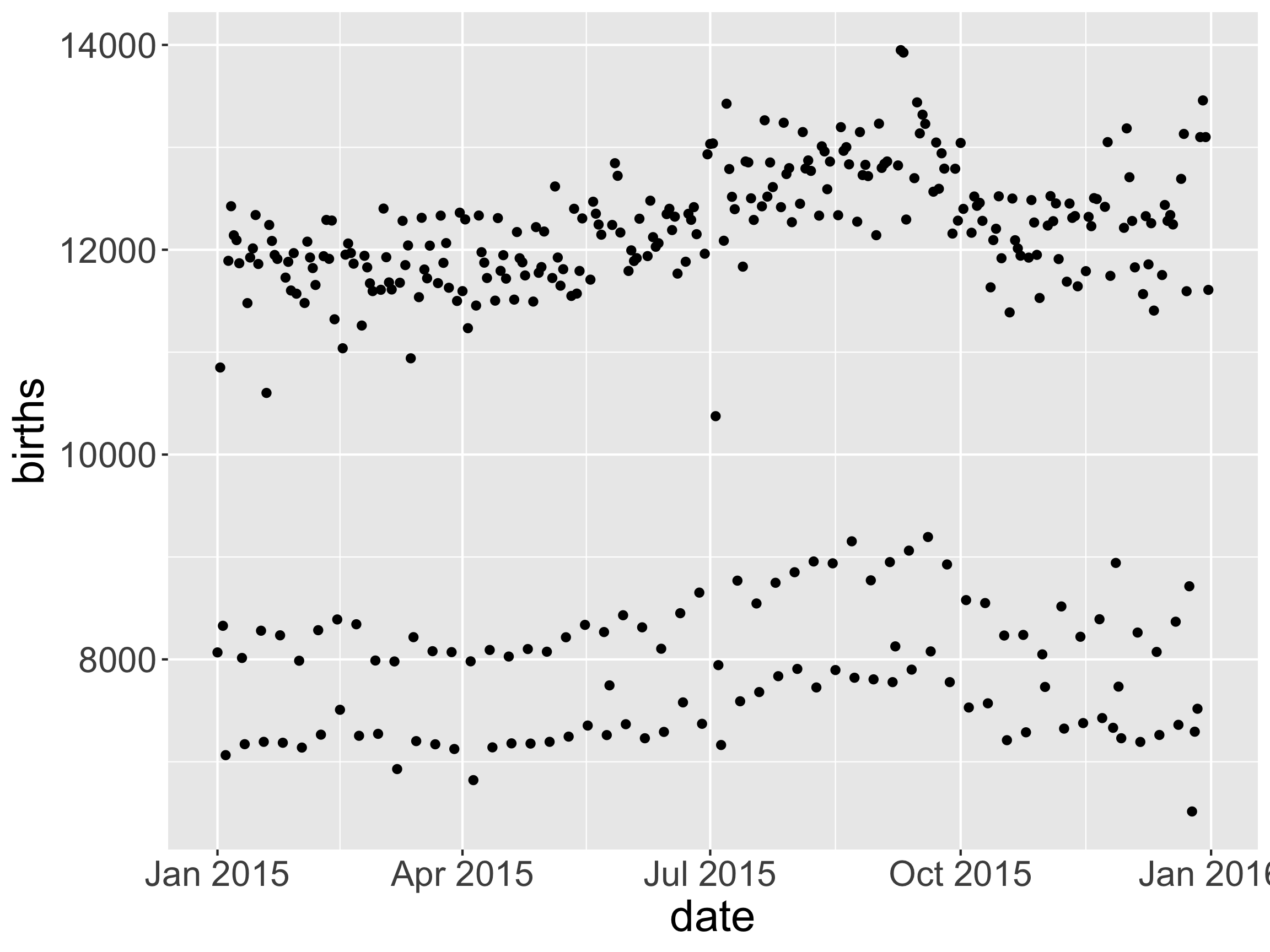
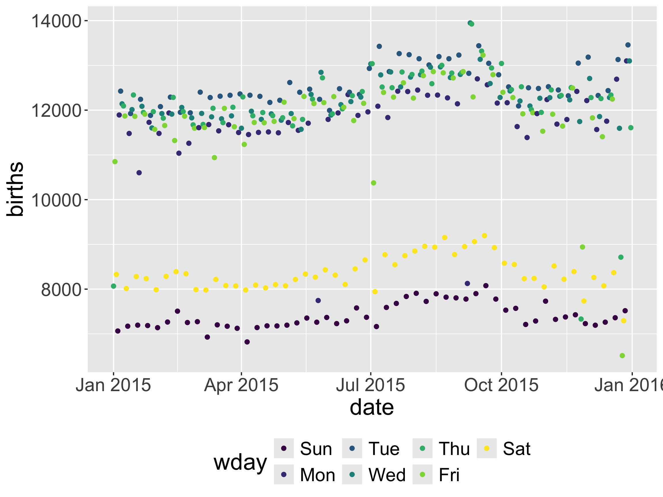
Example: Over the course of a year, how does the daily number of births vary?

- What patterns do you see?
Example
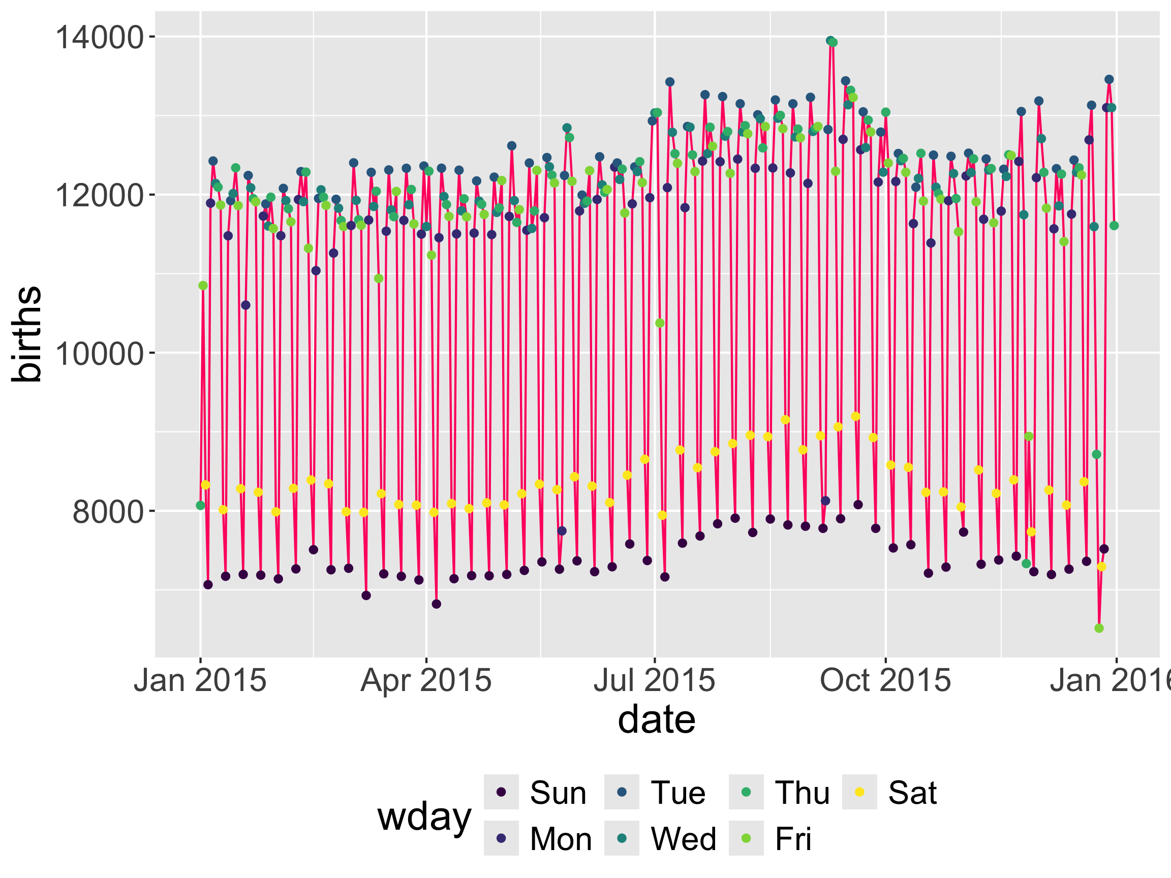
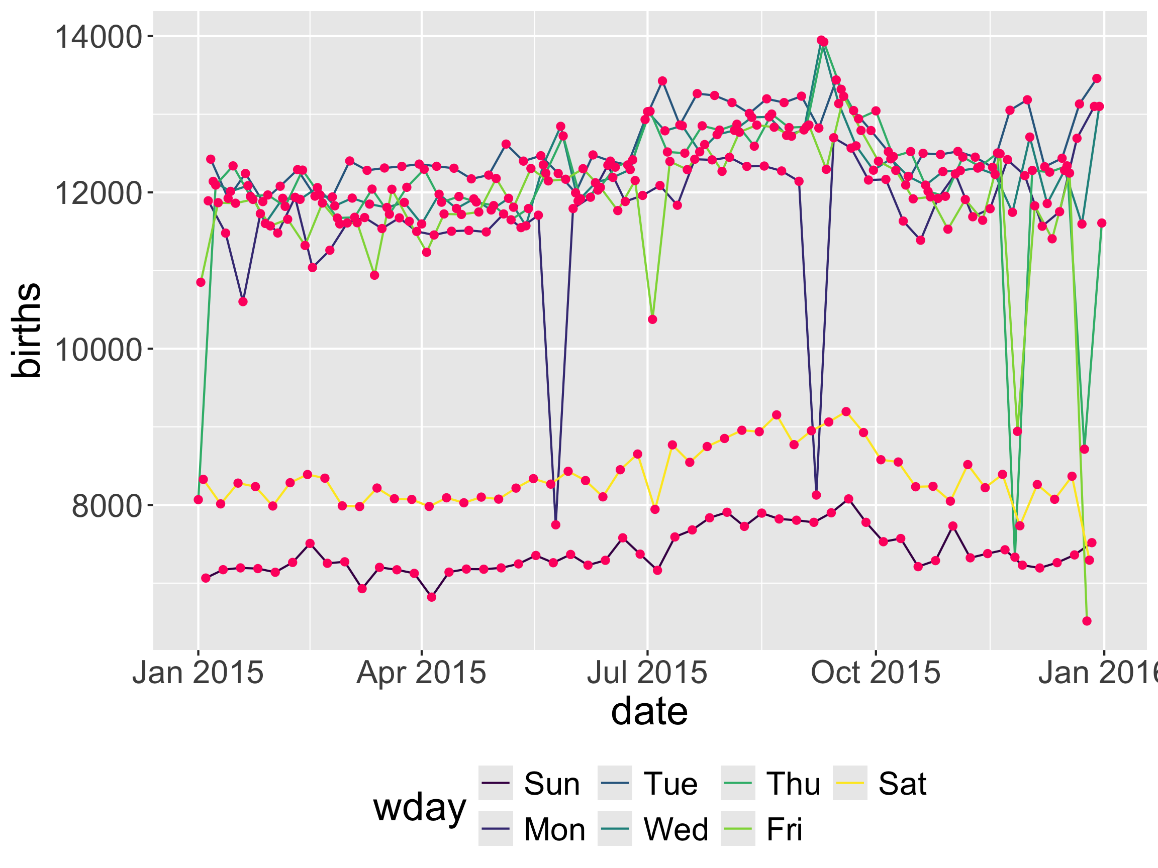
Example: Cycles related to day of the week?
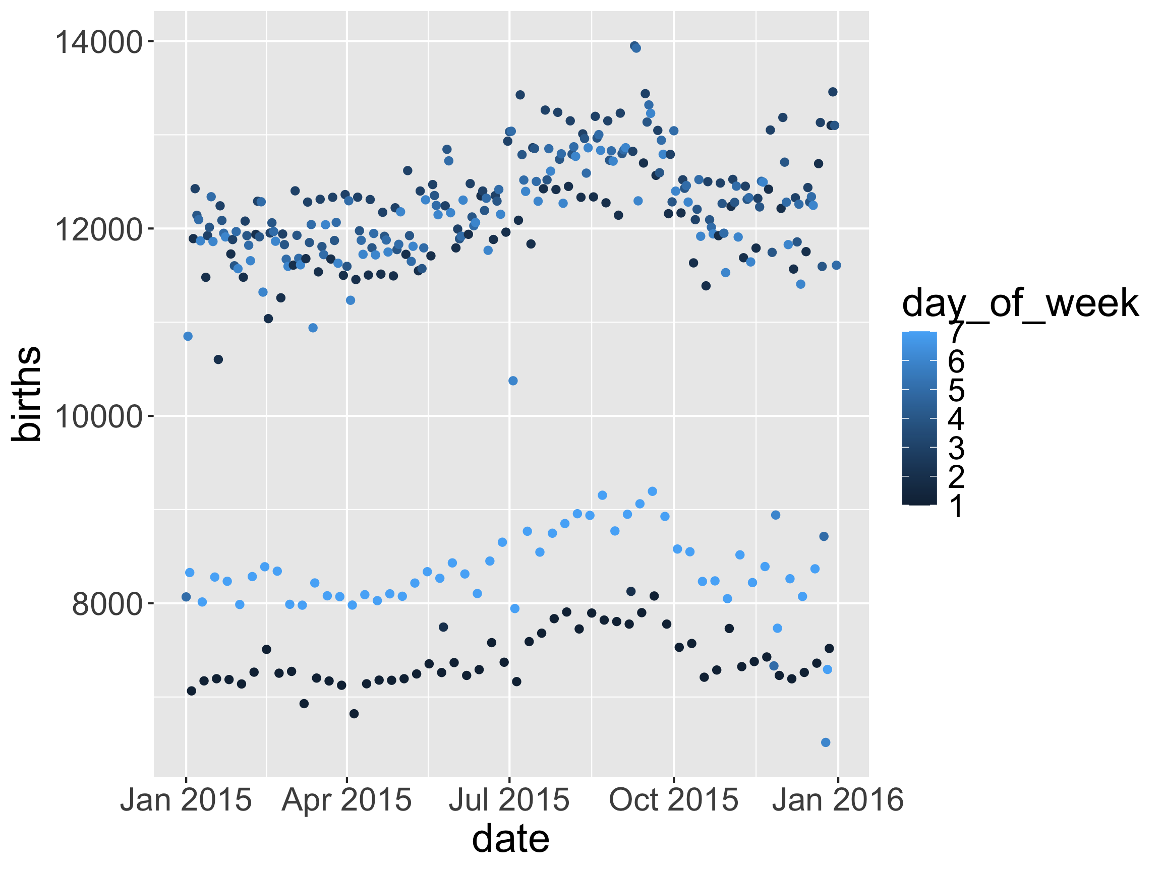
- Additional aesthetic:
- Why is this not quite what we want? What do we want?
- What happened to the aspect ratio when we added the legend?
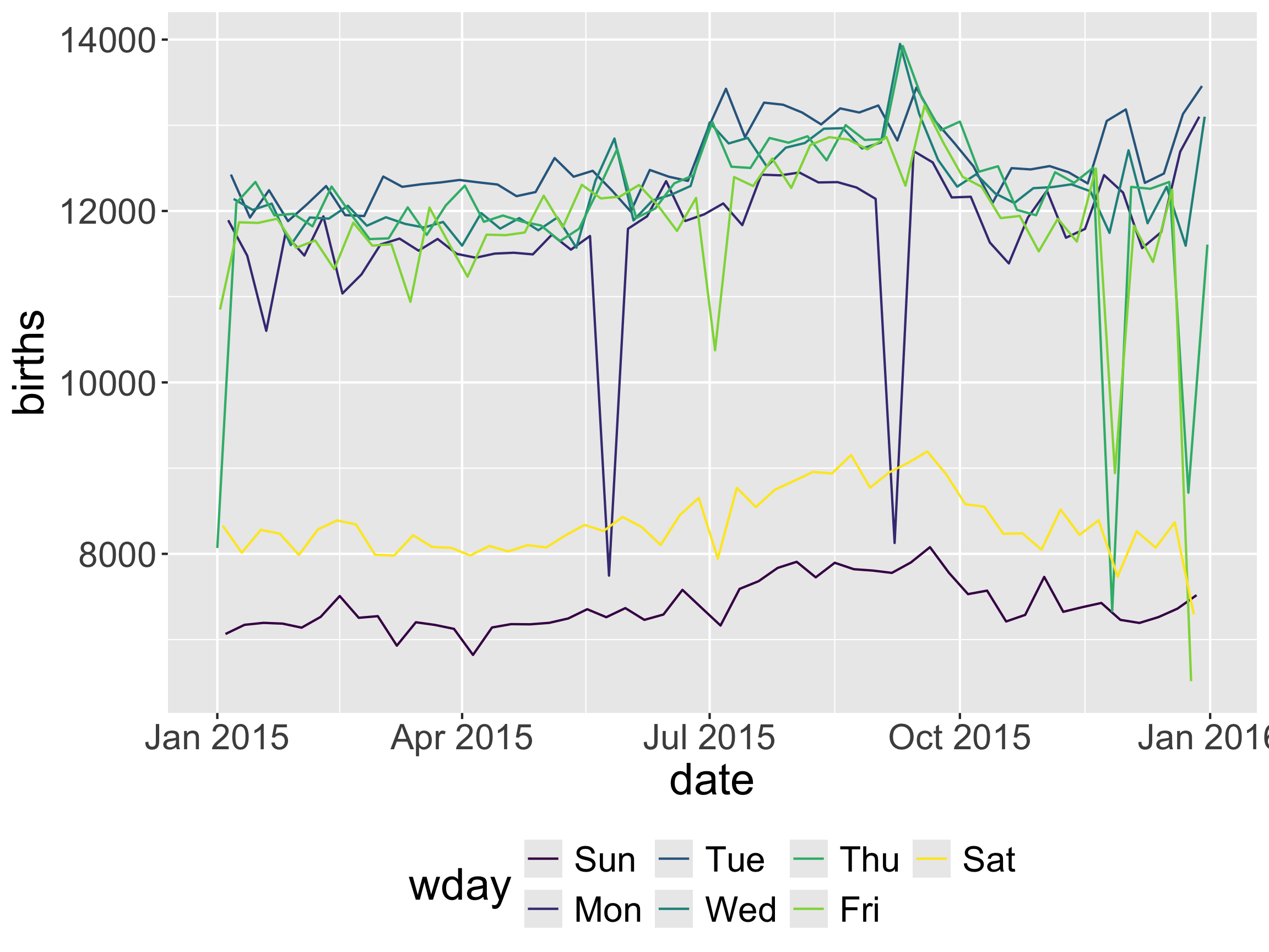
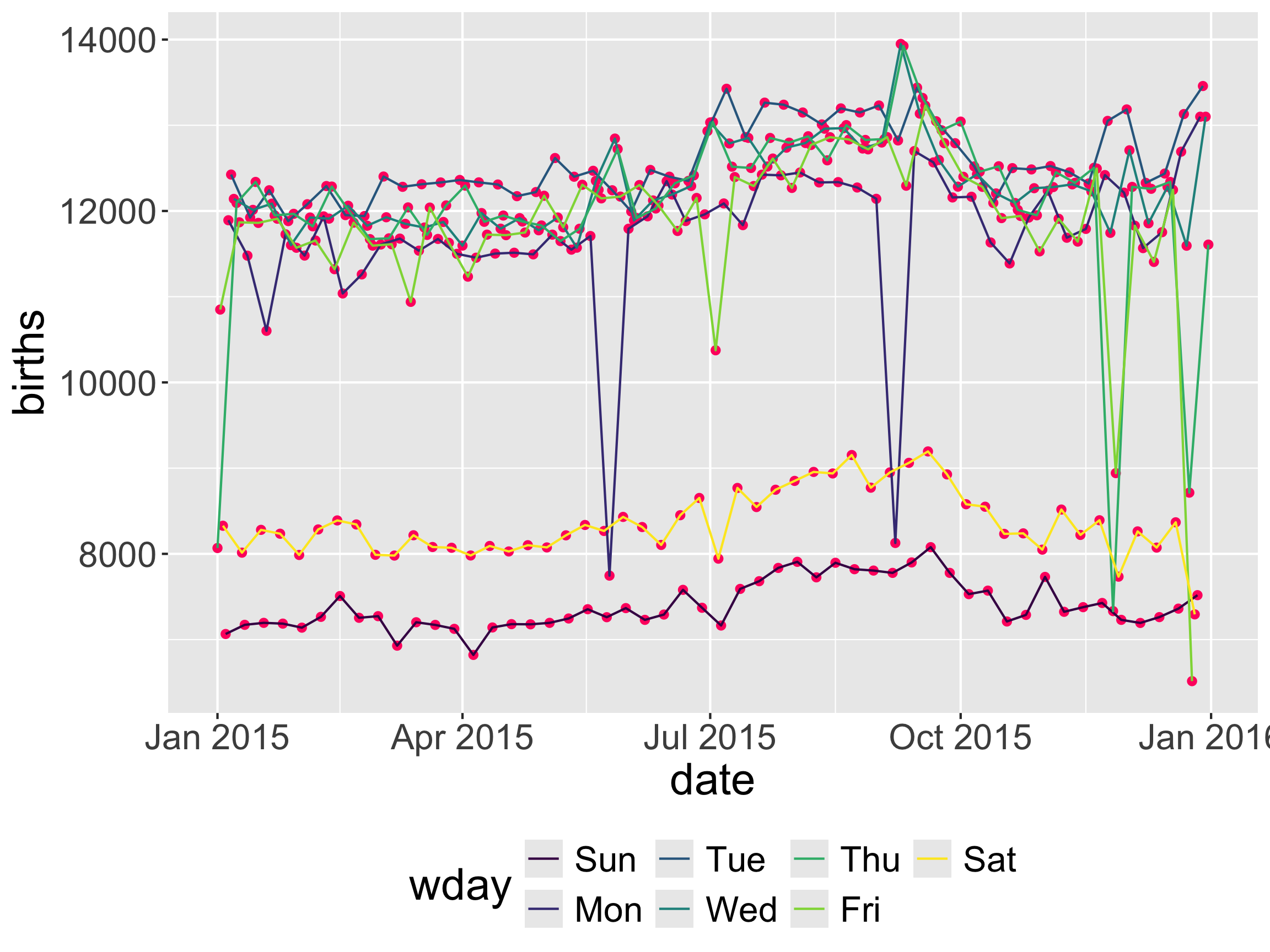
Example: Cycles related to day of the week?
Positioning the legend on the bottom of the graph helped give us a nicer aspect ratio.
What if we want to see the direction that the number of births take over time for each day of the week?
- New visual cue/
geom?
- New visual cue/
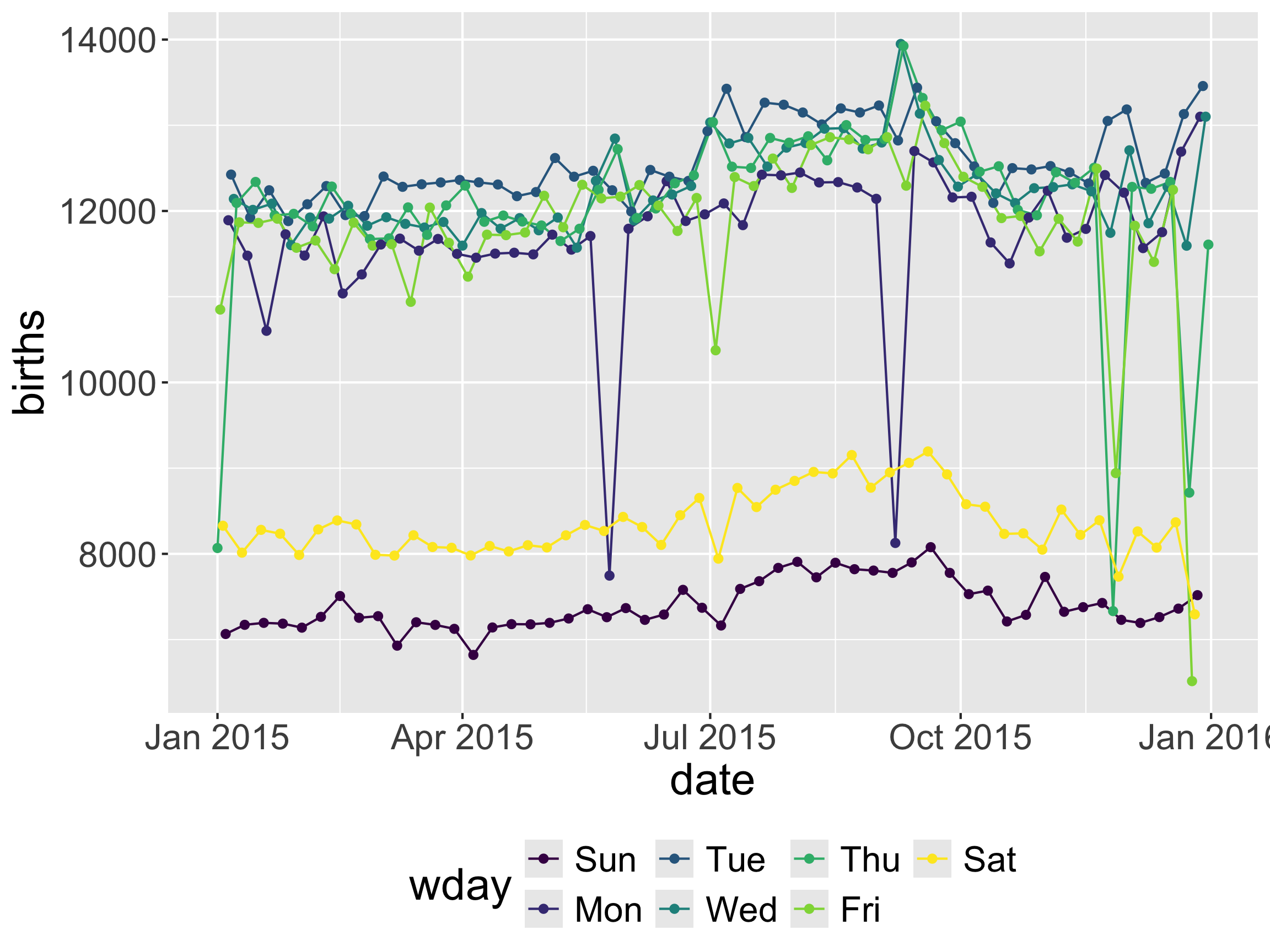
Example
- What if we want visual cues for both position and direction?
Example
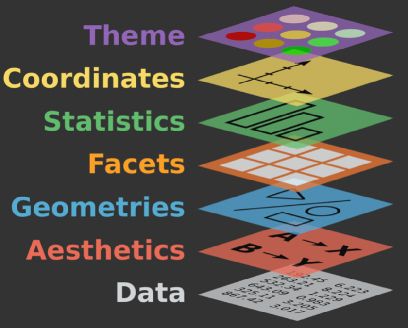
Coordinate System Layer
How did this new layer change our plot?
What if we want all the points to be colored “midnightblue”?
Setting instead of Mapping
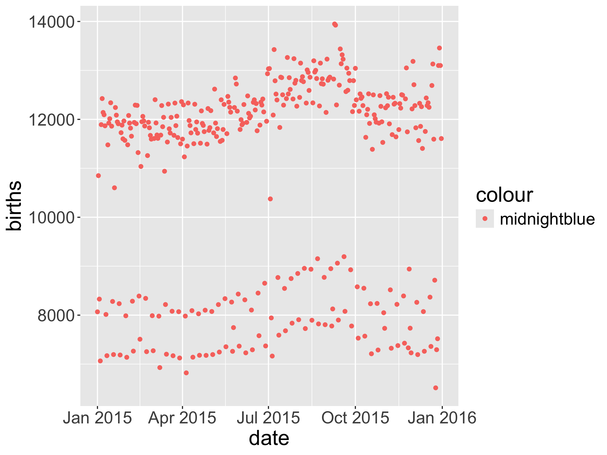
Setting instead of Mapping
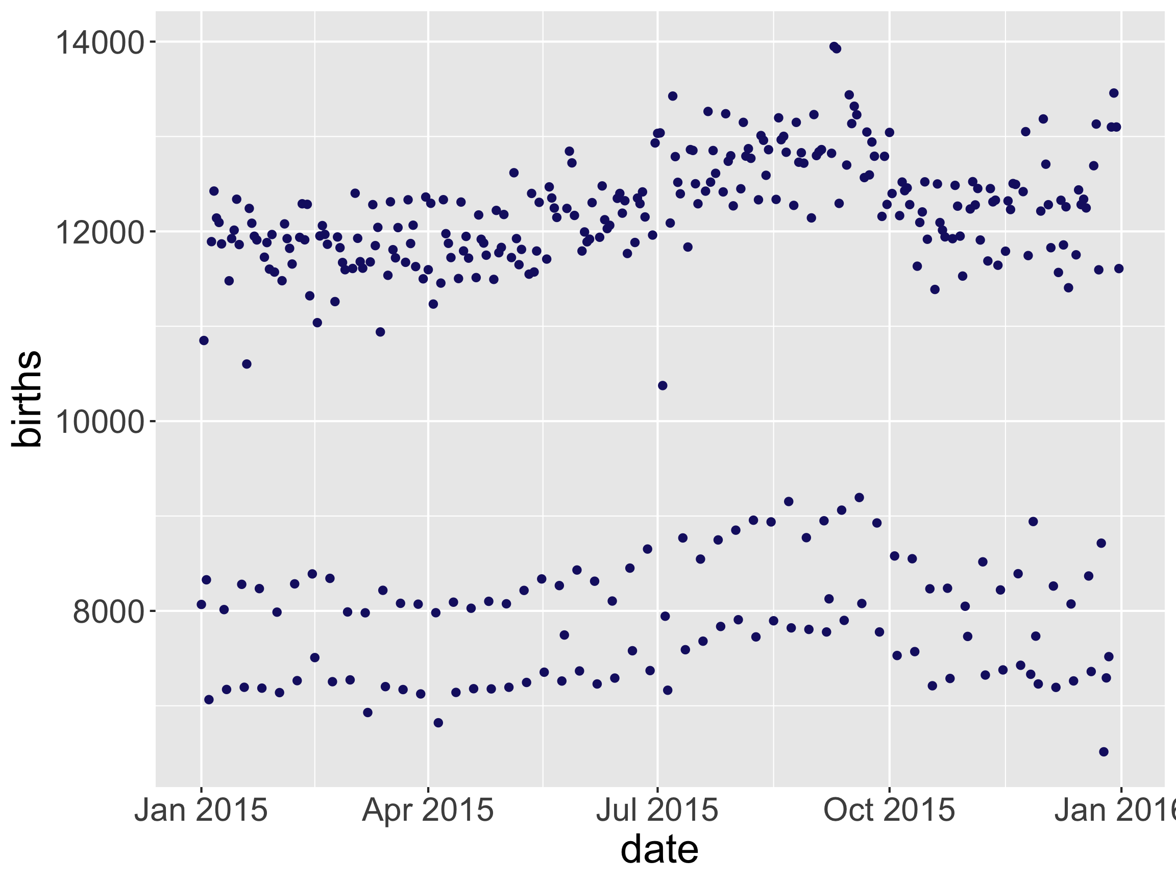
- If you want to set an aesthetic to a specific value (instead of mapping the aesthetic to a variable), do so in the
geom_--()function.
Layer order (sometimes) matters
Layer order (sometimes) matters
Layer order (sometimes) matters
- Inheriting aesthetics discussion.
Adding Curve(s)
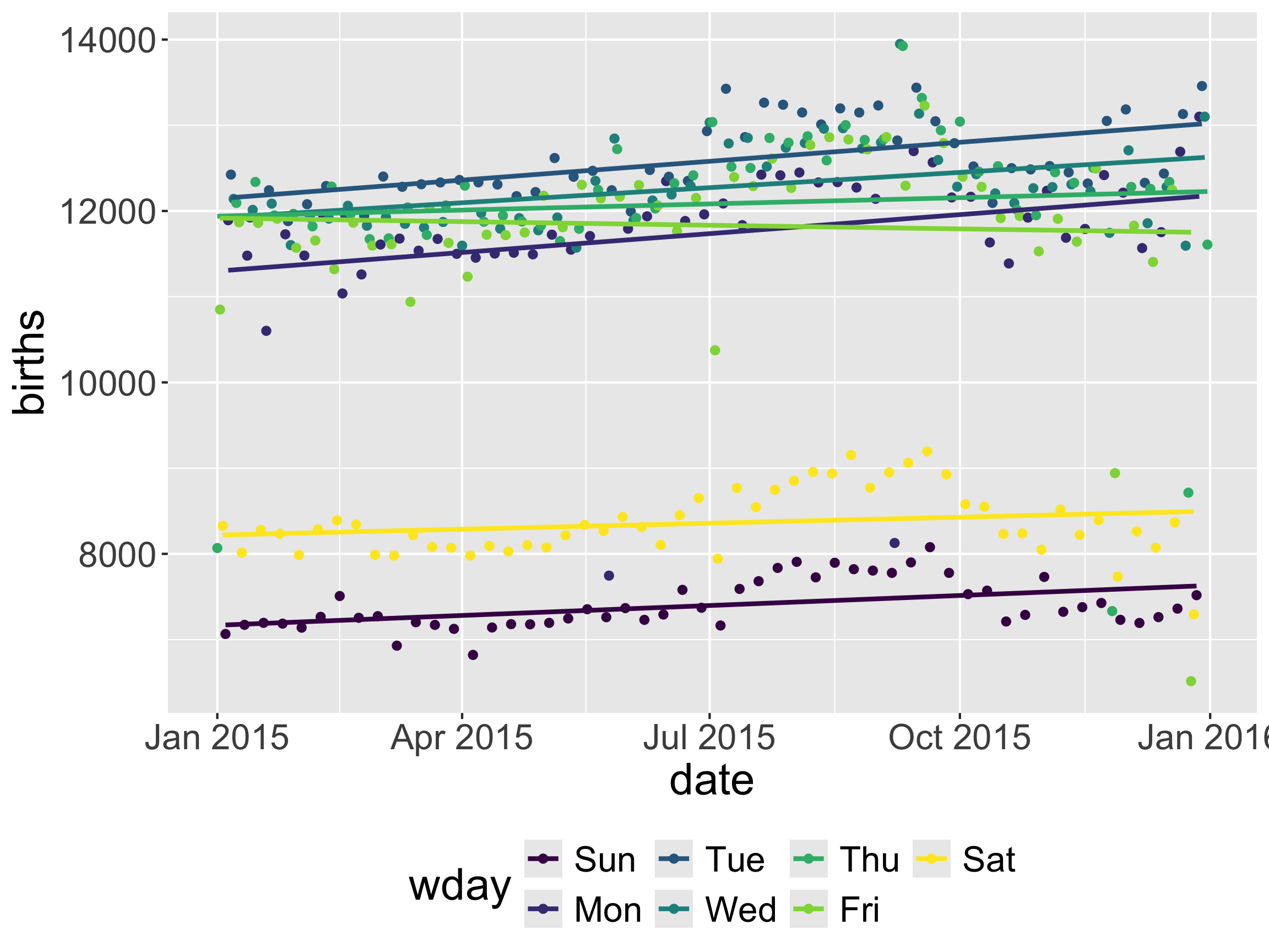
- Does a multiple linear regression line(s) capture the trend?
Adding Curve(s)
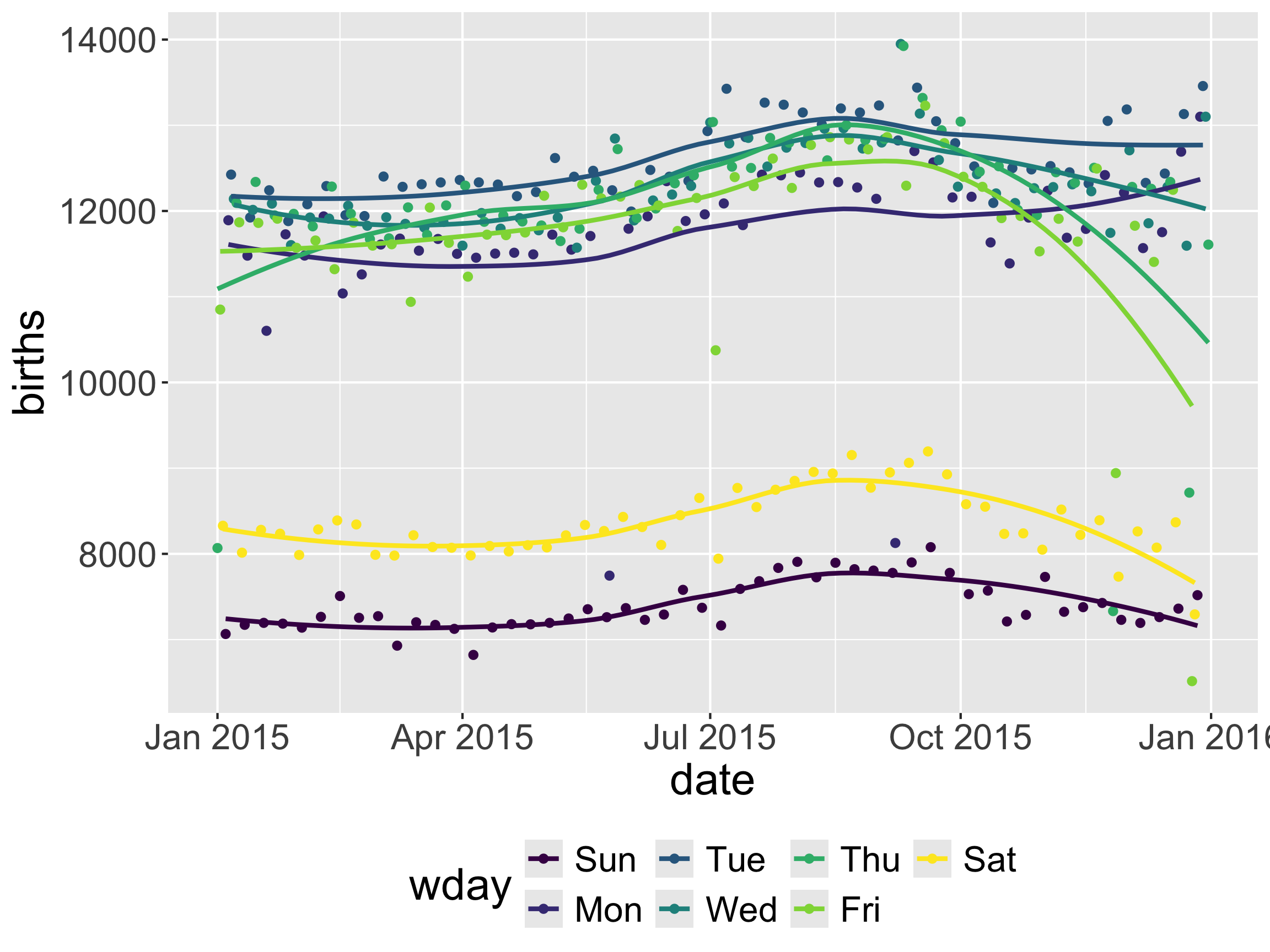
- The default LOESS smoother usually does a reasonable job.
Adding Curve(s)
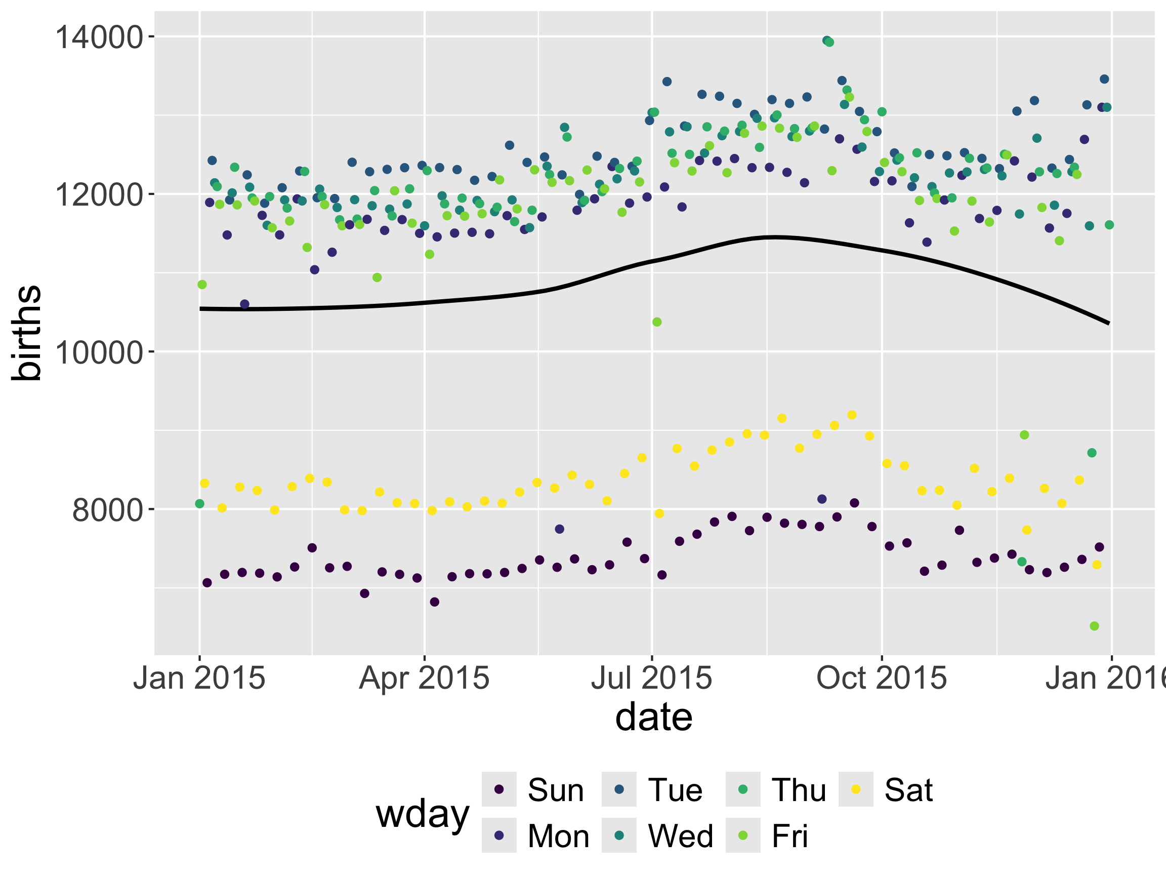
What happened?
Inheriting aesthetics discussion.
Amounts: geom_bar
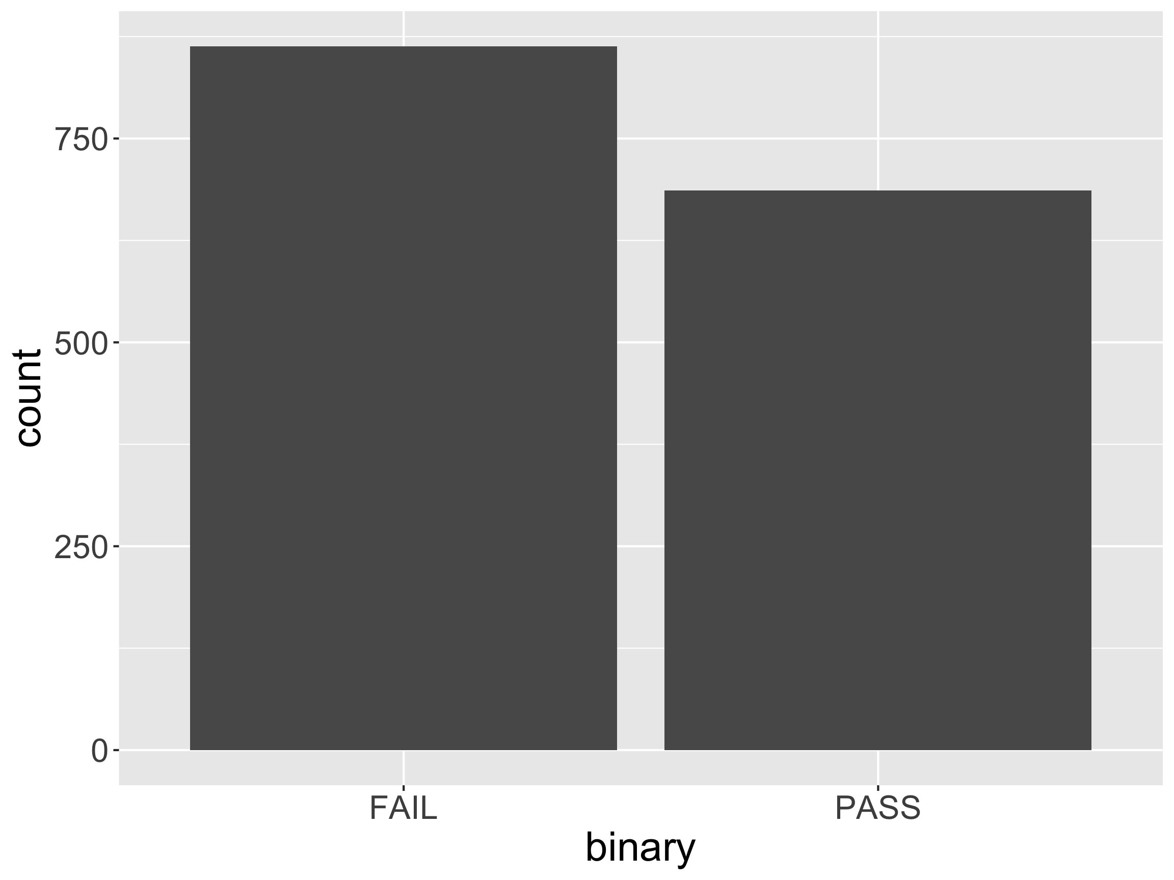
- Verbalize the mapping of data to geom_bar().
- How is this mapping different from geom_point()?
Another option: geom_col

geom_point again
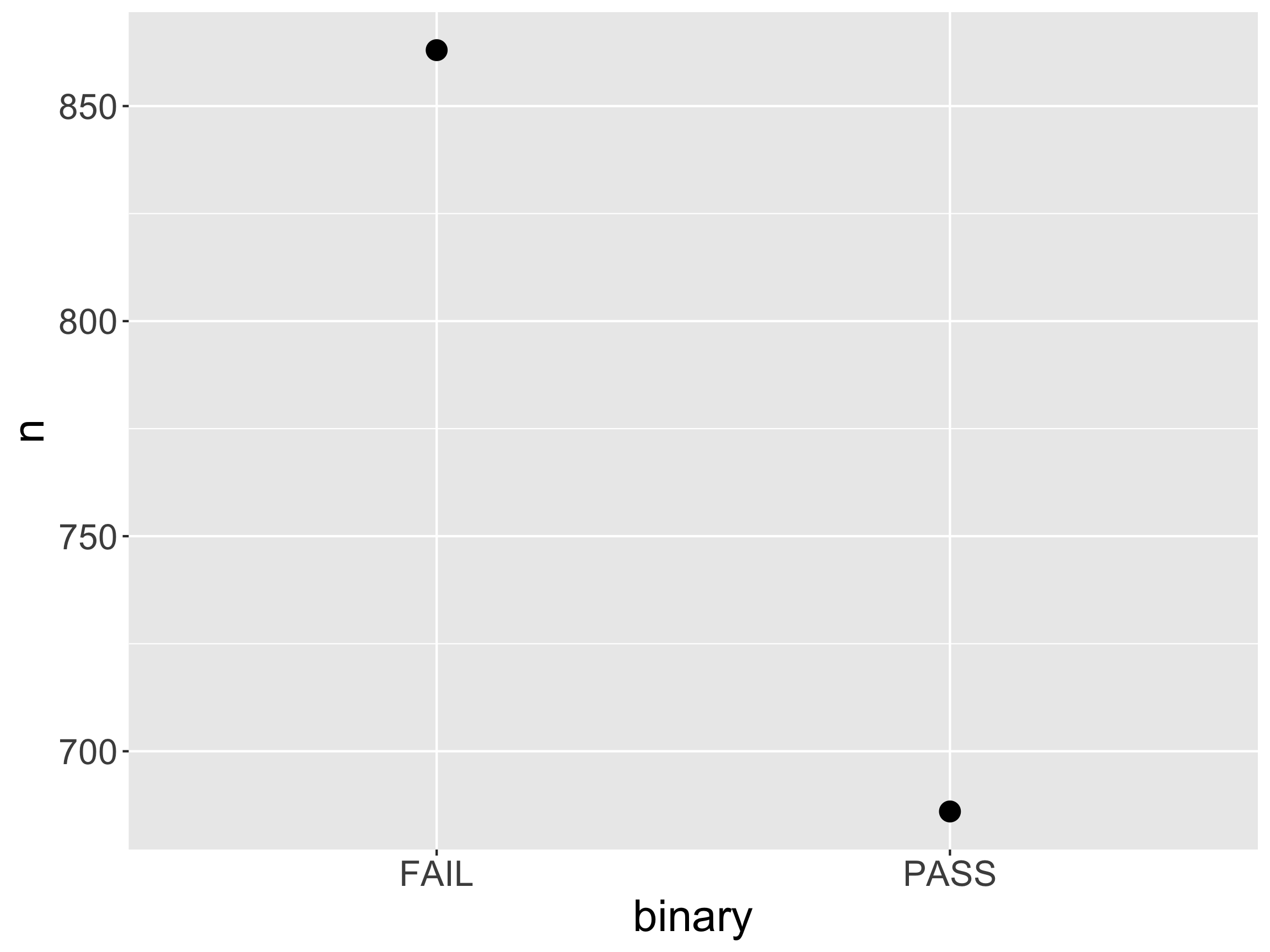
- If you are worried about the data-ink ratio…
geom_point + geom_segment
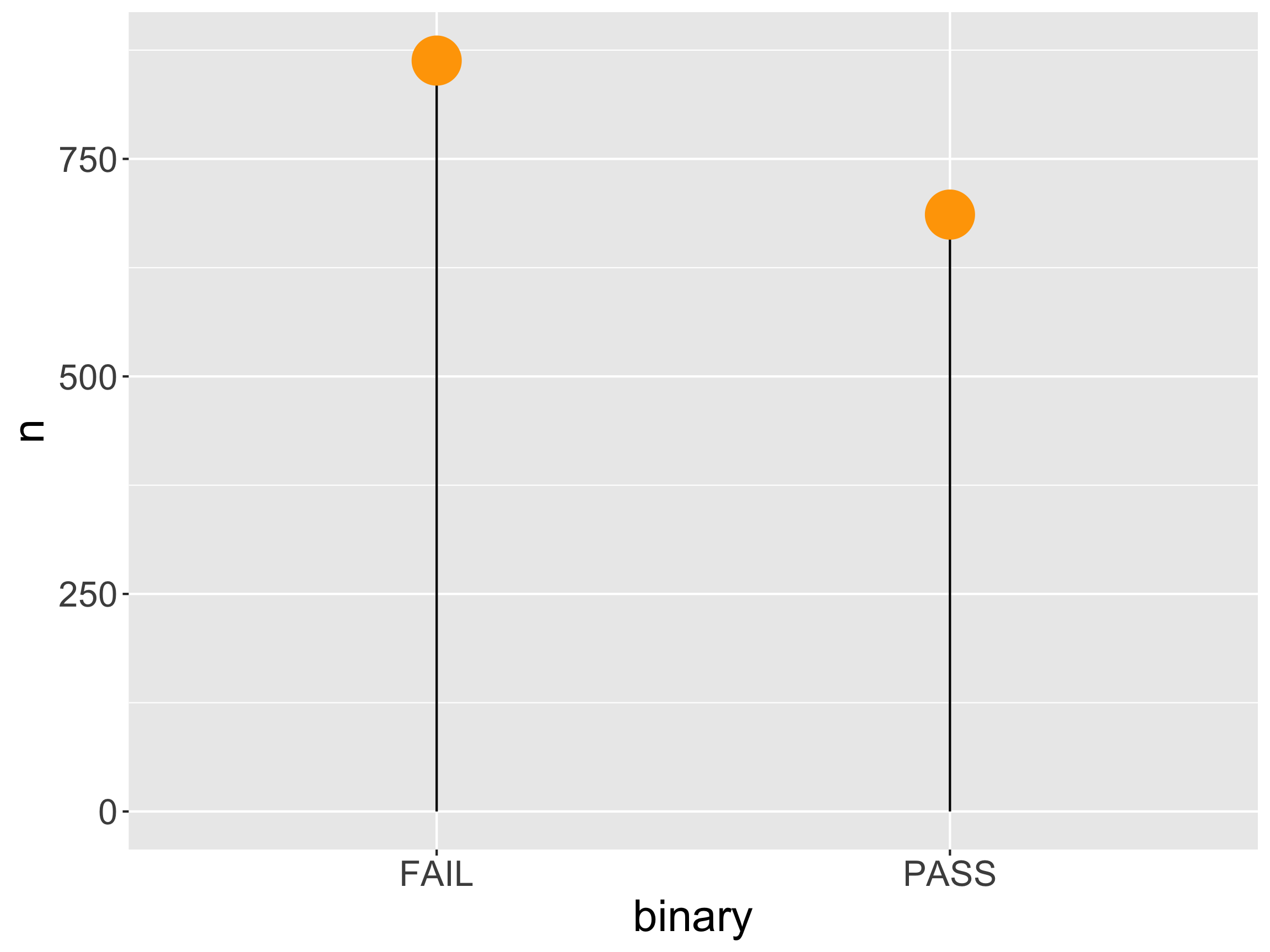
- Lollipop chart: compromise?
Two categorical variables: geom_bar
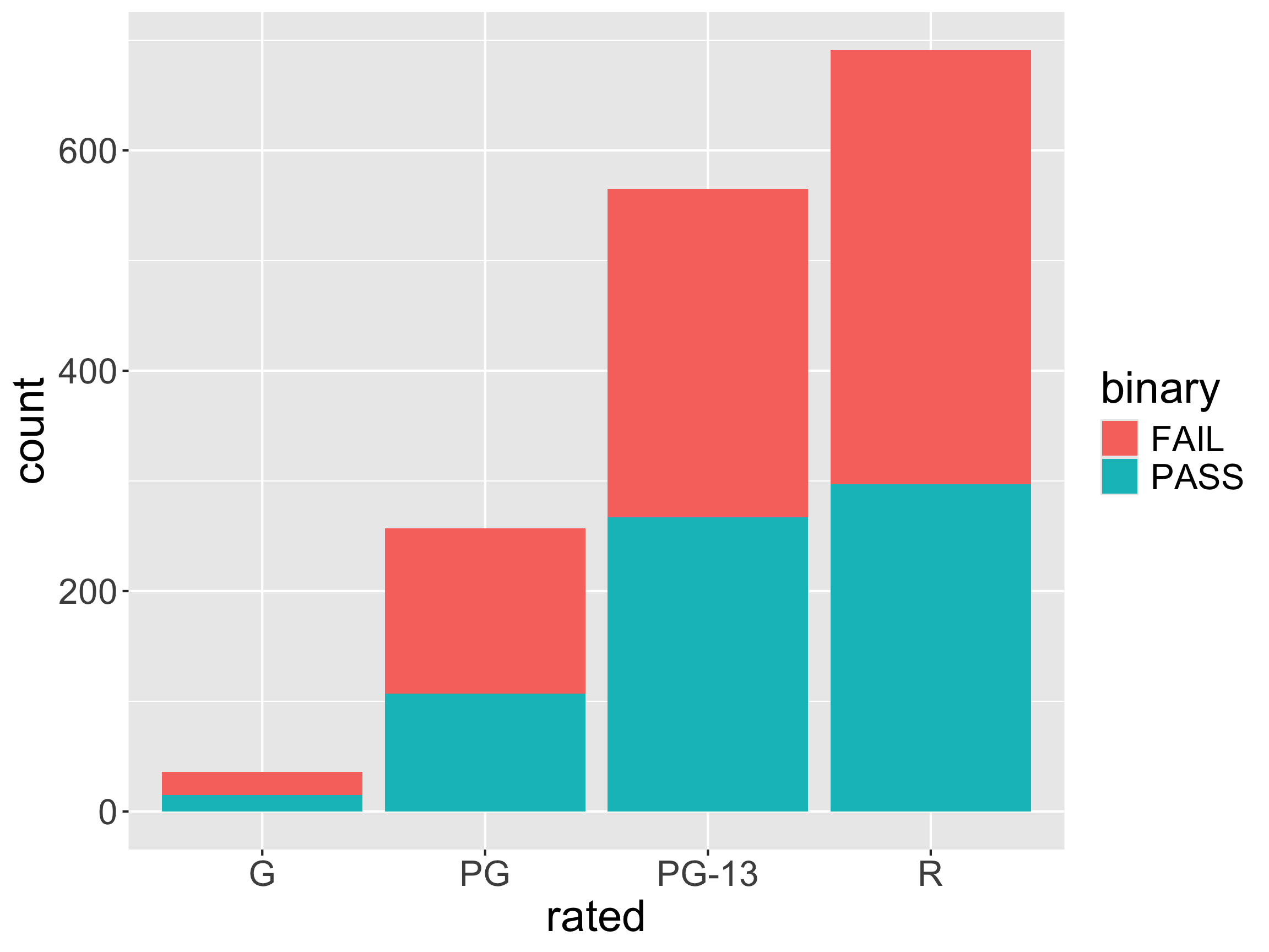
- Describe the mapping.
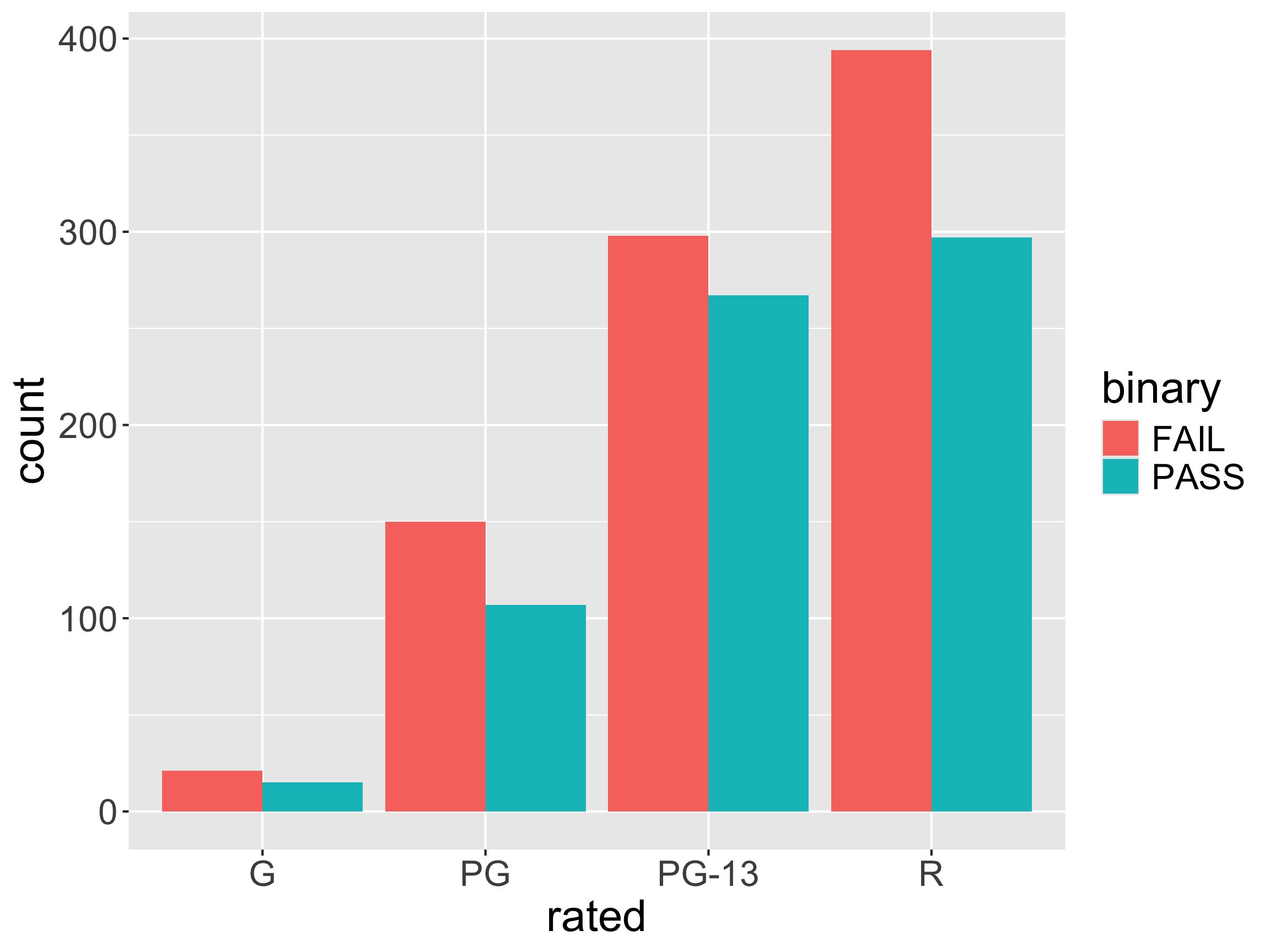
Two categorical variables: geom_bar
- Describe the mapping.
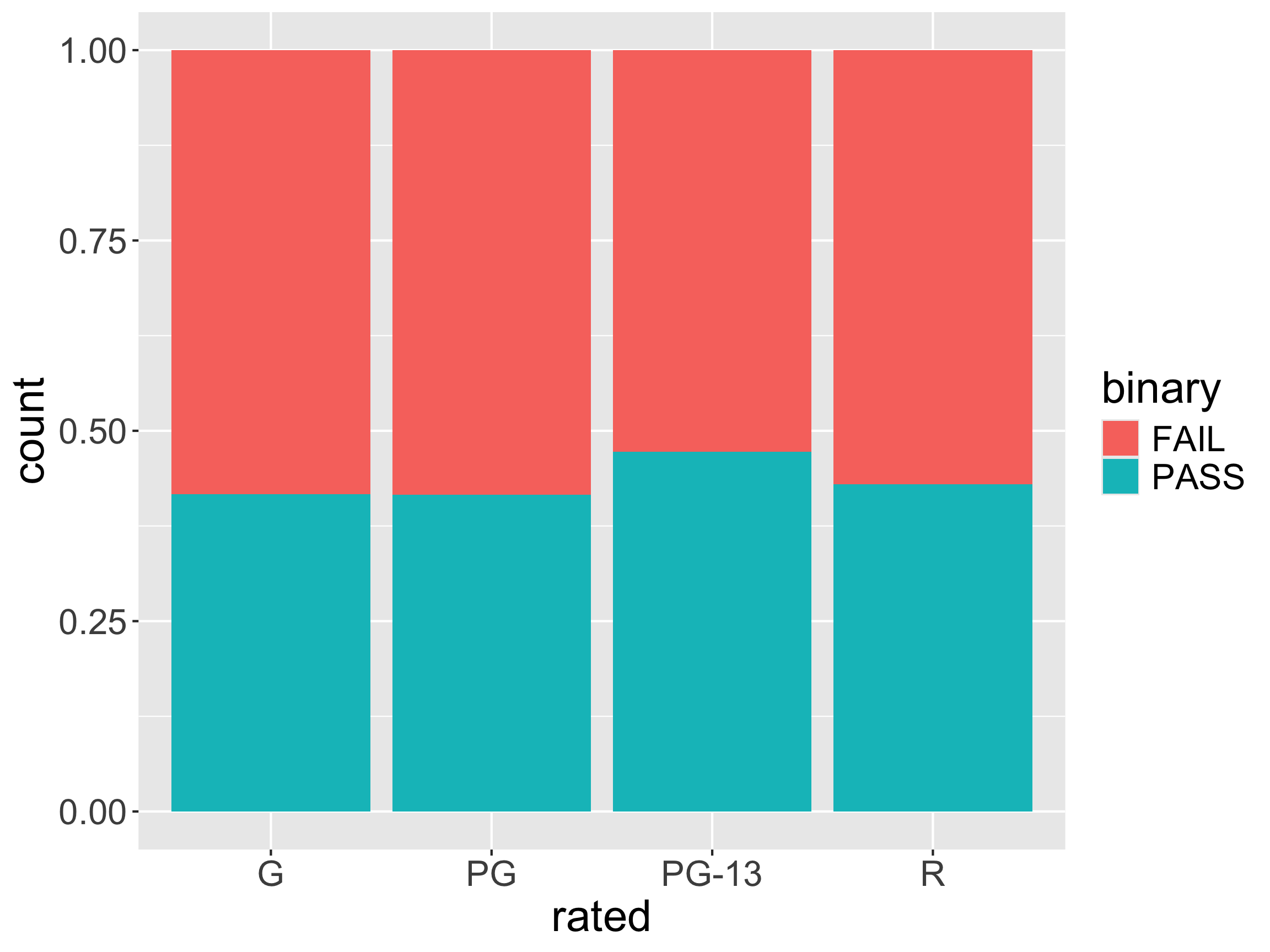
Two categorical variables: geom_bar
- Describe the mapping.
Two categorical variables: geom_tile
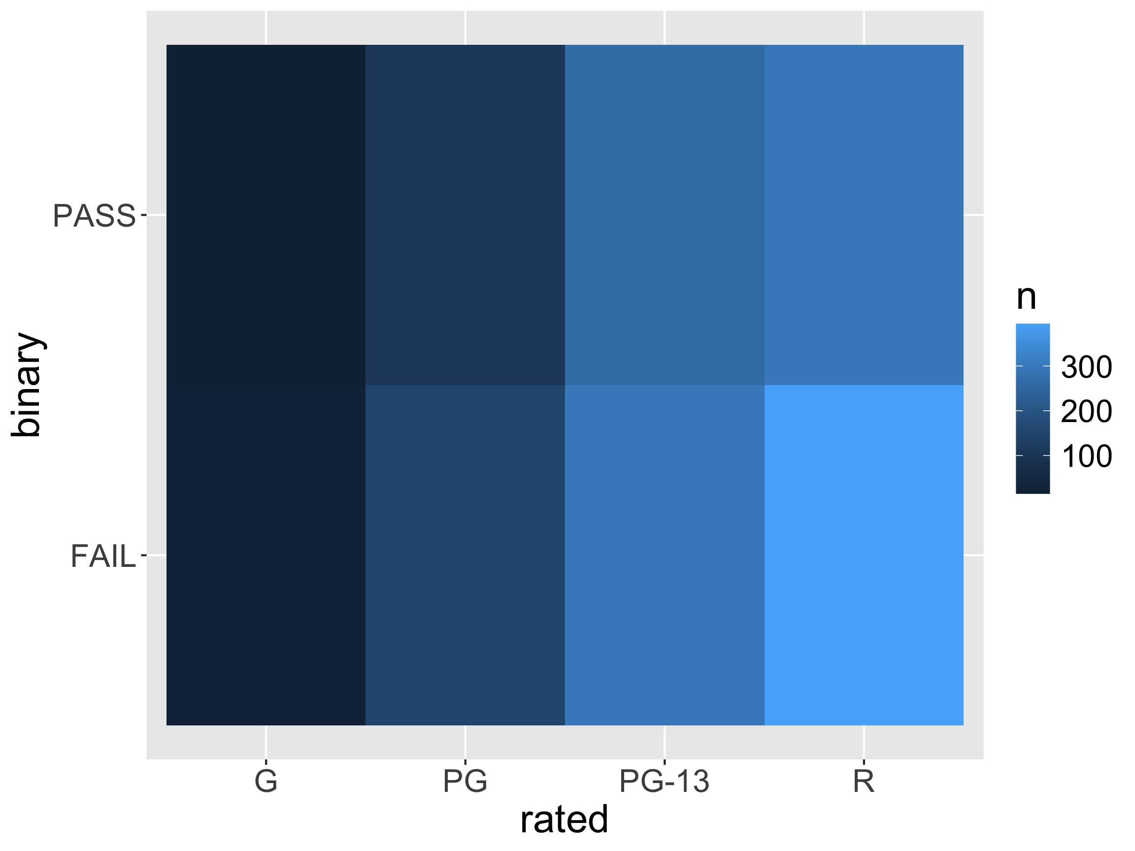
- Describe the mapping.
Two categorical variables: geom_tile
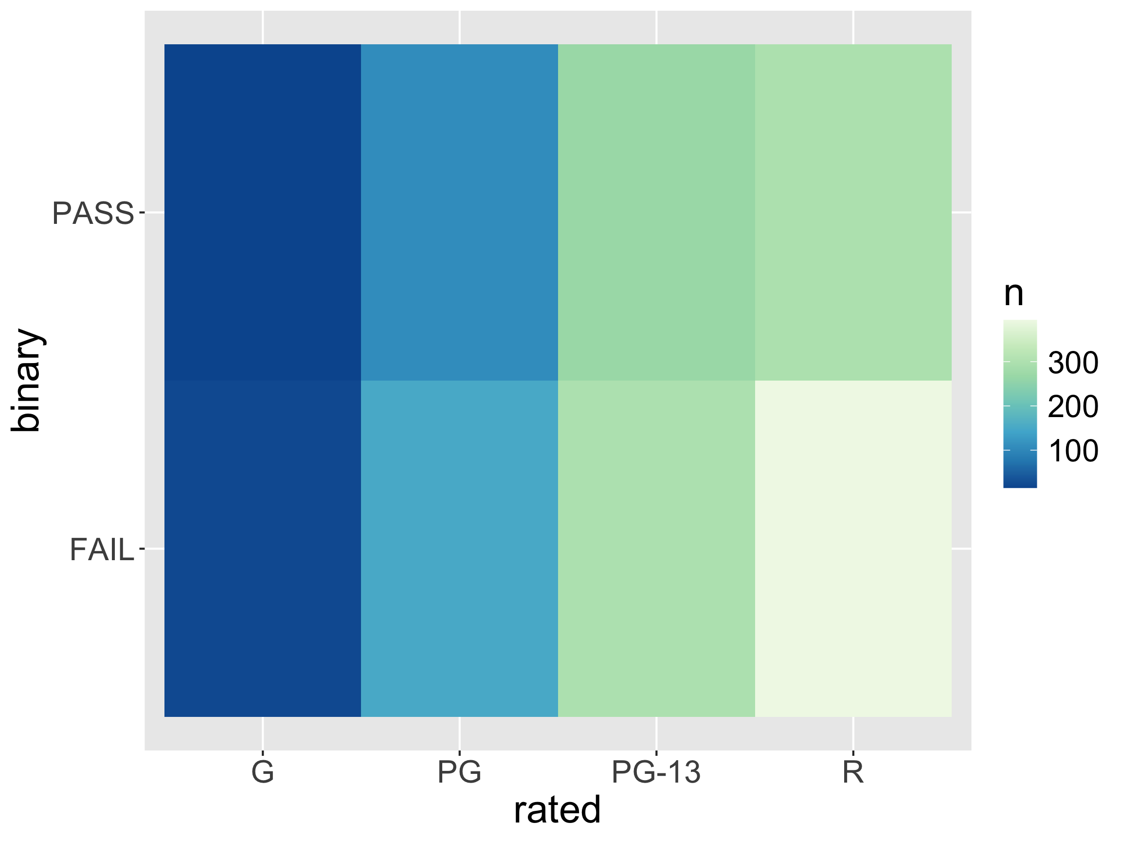
- Change the
fillscale!
Can display more than frequencies!
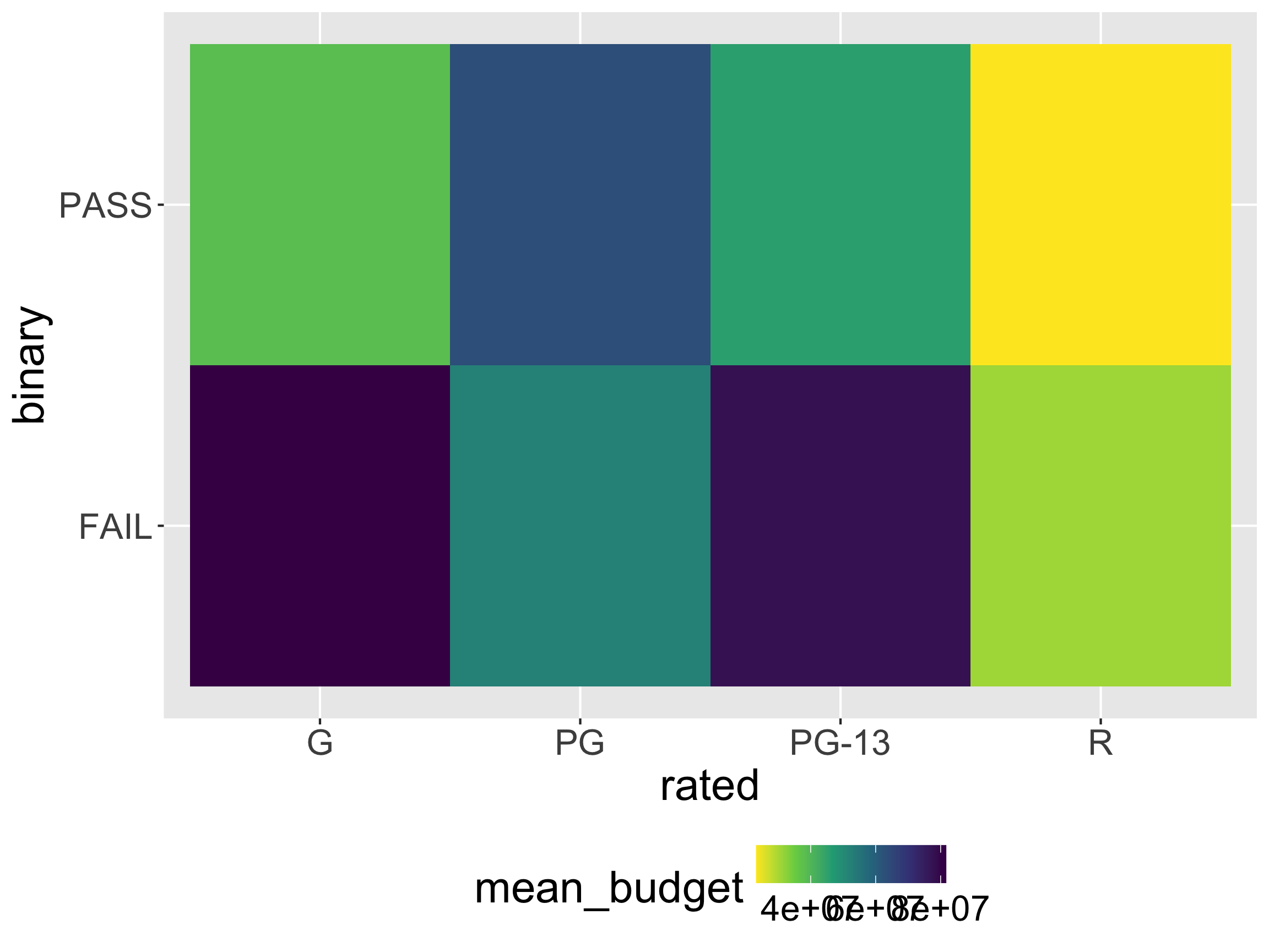
Can display more than frequencies!
options(scipen = 999) # turn off scientific notation

movies_ag <- group_by(movies,
                      rated, binary) %>%
  summarize(mean_budget = mean(budget))

ggplot(data = movies_ag,
       mapping = aes(x = rated,
                     y = binary,
                     fill = mean_budget)) +
  geom_tile() +
  scale_fill_viridis_c(direction = -1,
                       guide = guide_colorbar(angle = 90)) +
  theme(legend.position = "bottom")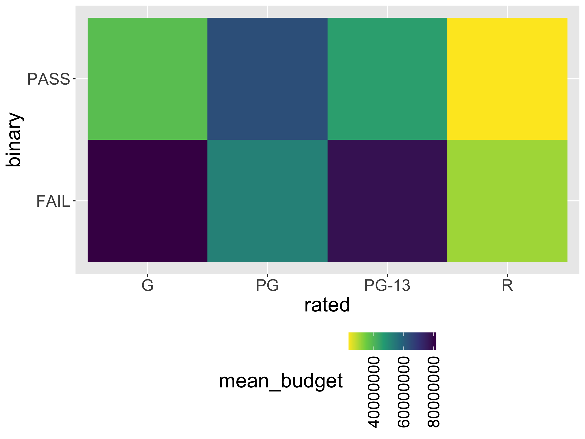
Distributions: geom_histogram
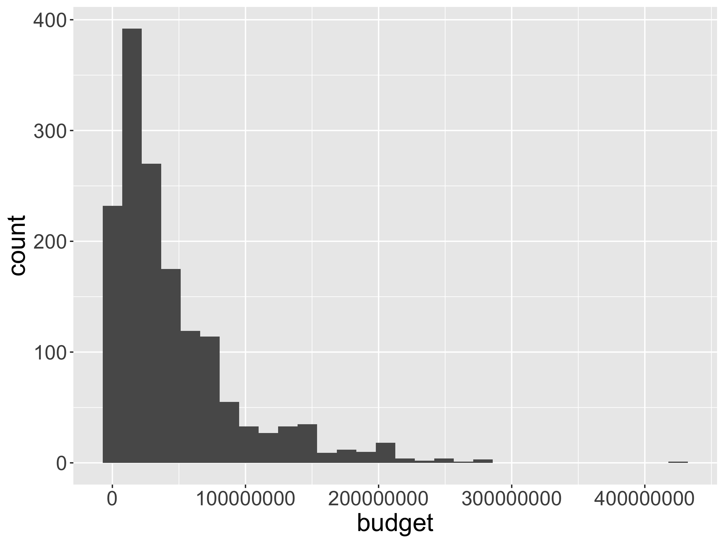
- Describe the mapping.
Distributions: geom_histogram
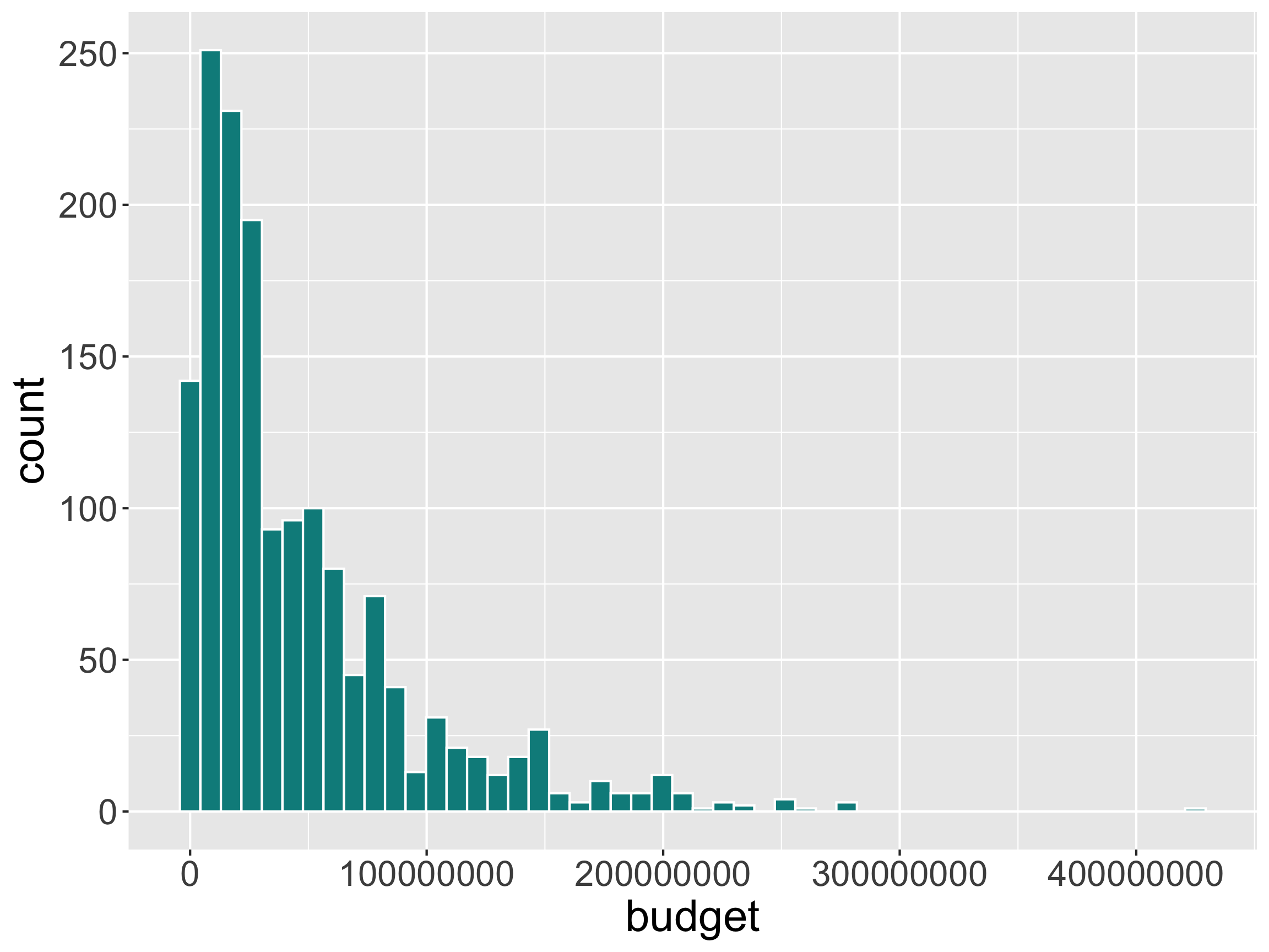
- Can modify the mapping via the
binwidthorbinsarguments
Distributions: geom_histogram
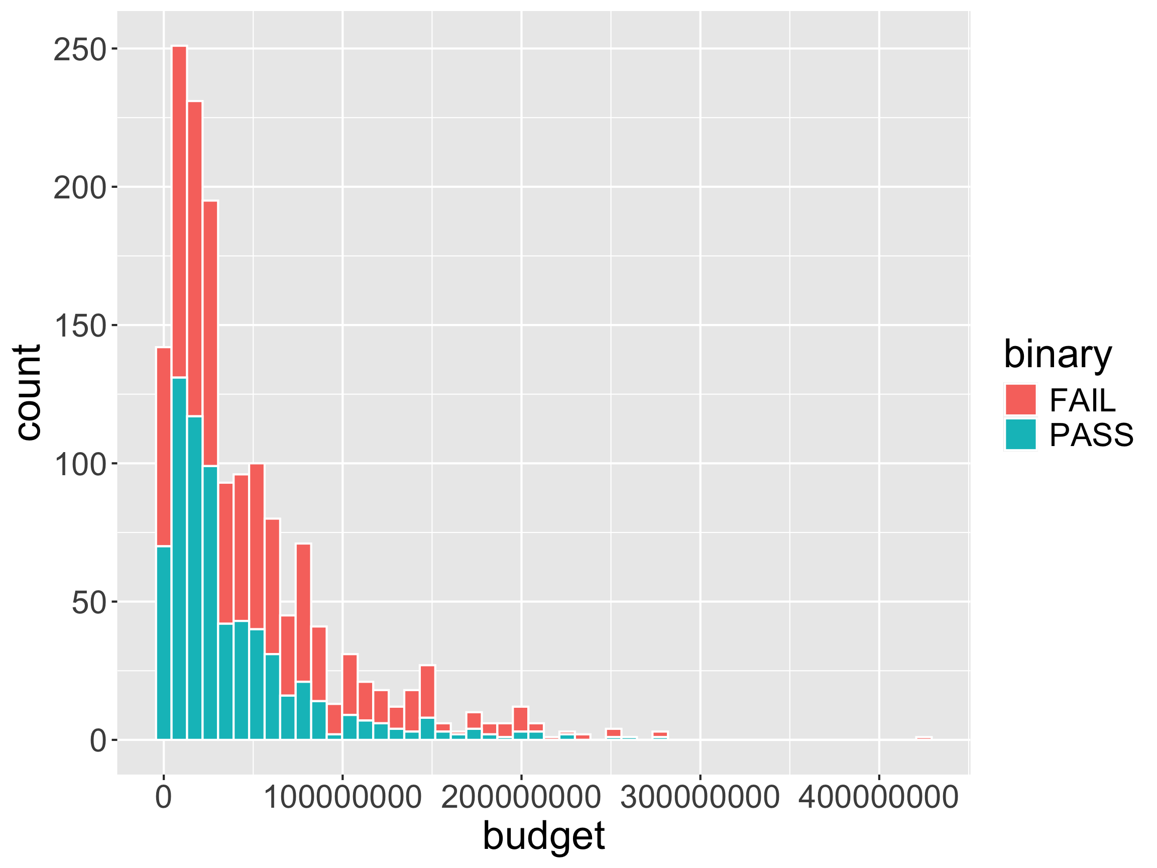
- What is problematic about this graph?
Distributions: geom_histogram
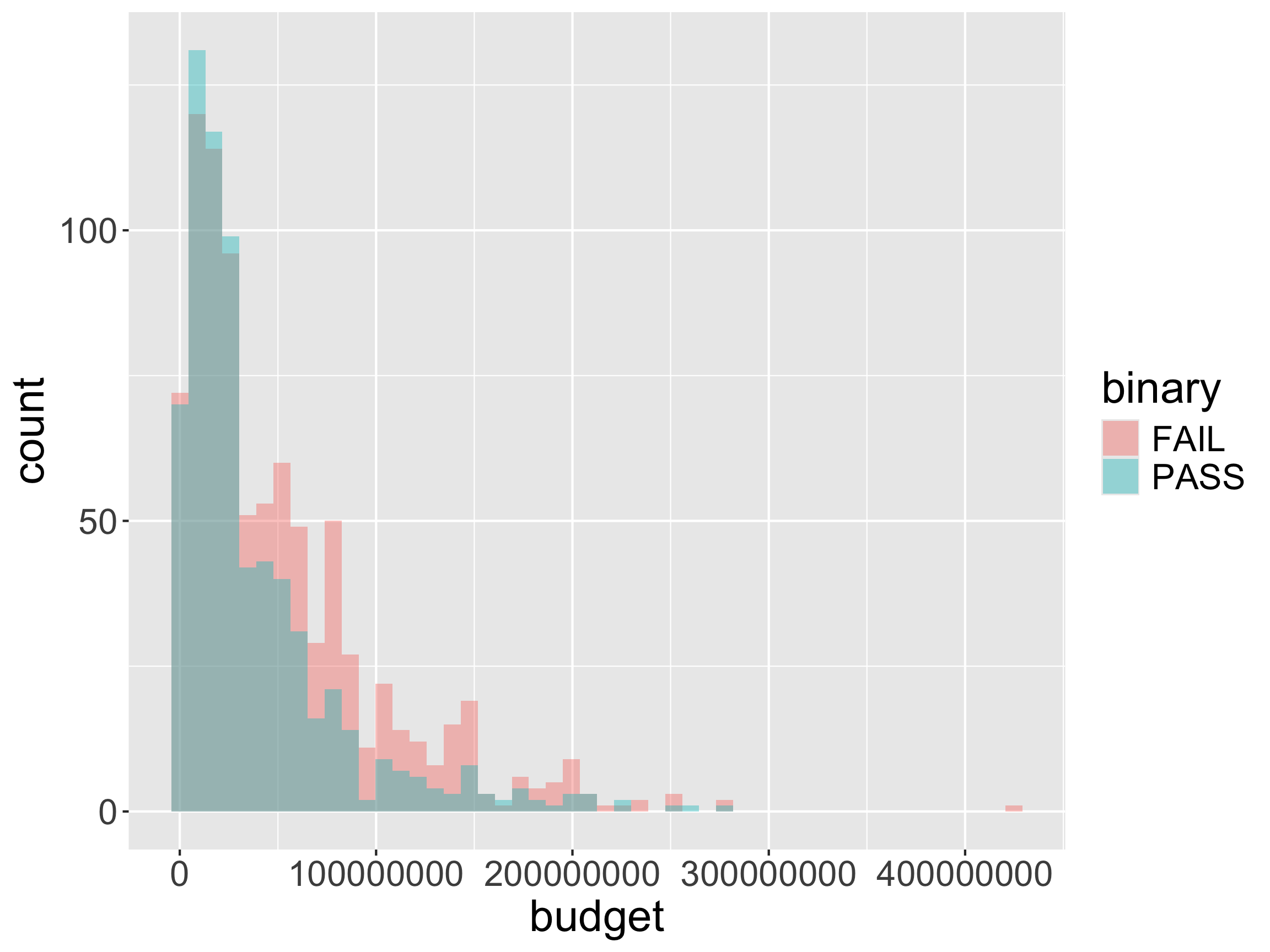
- Still problematic.
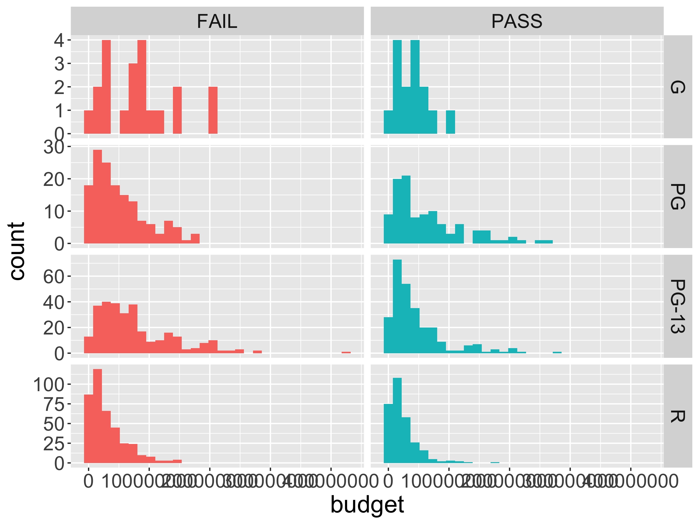
One option: Faceting
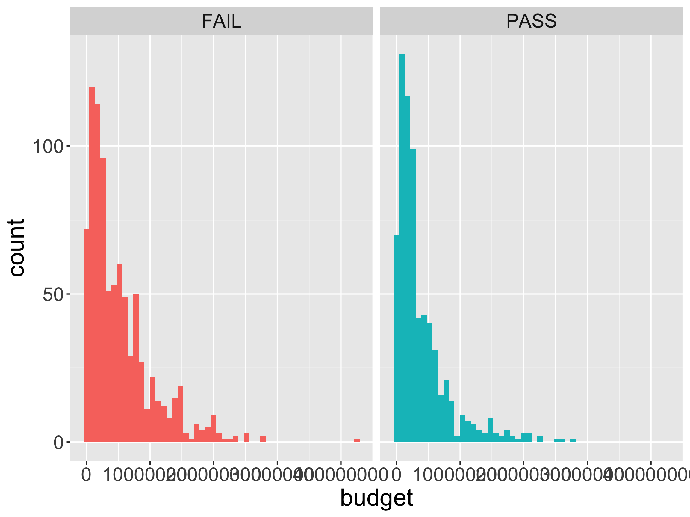
One option: Faceting
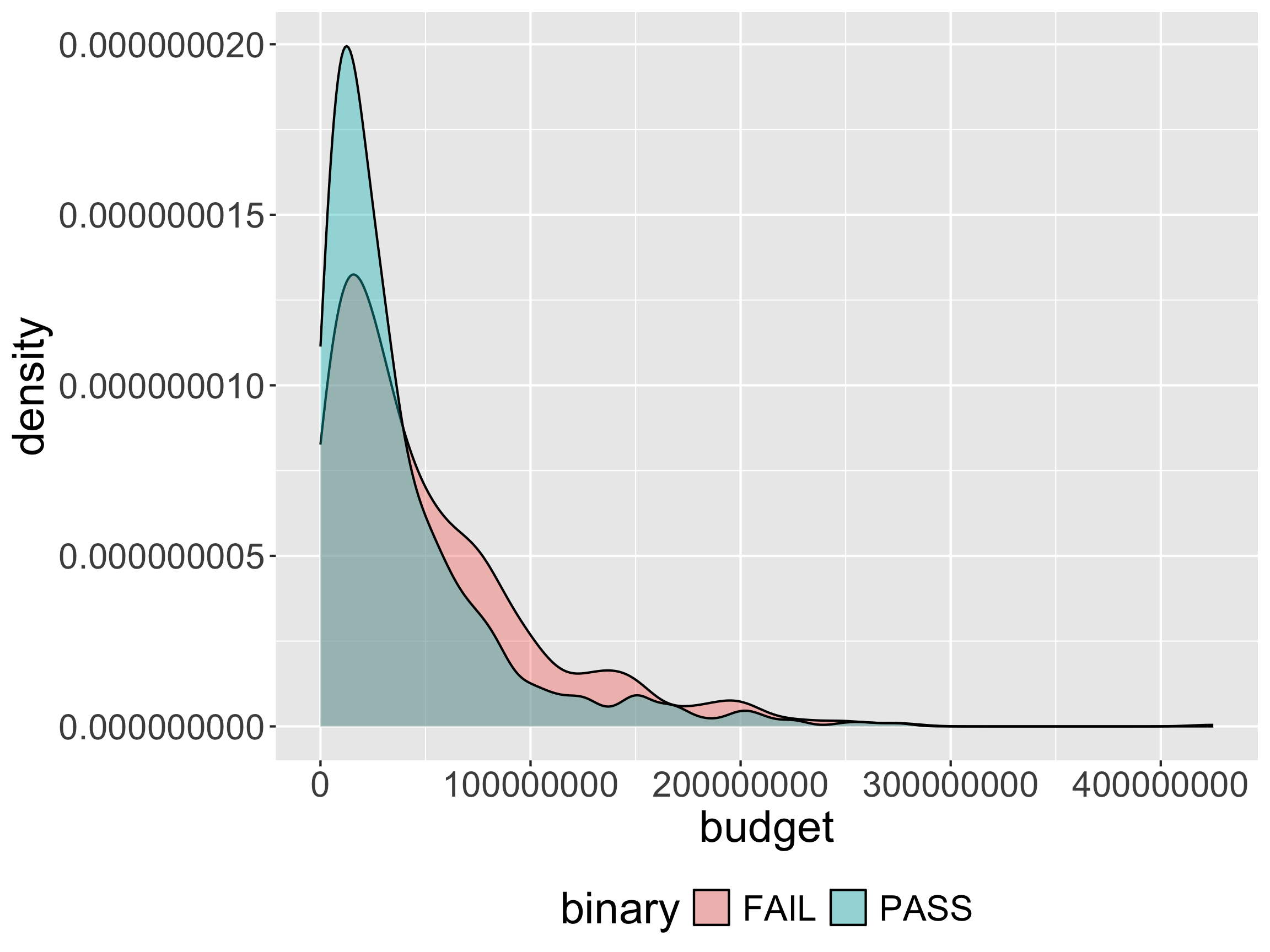
Another option: geom_density
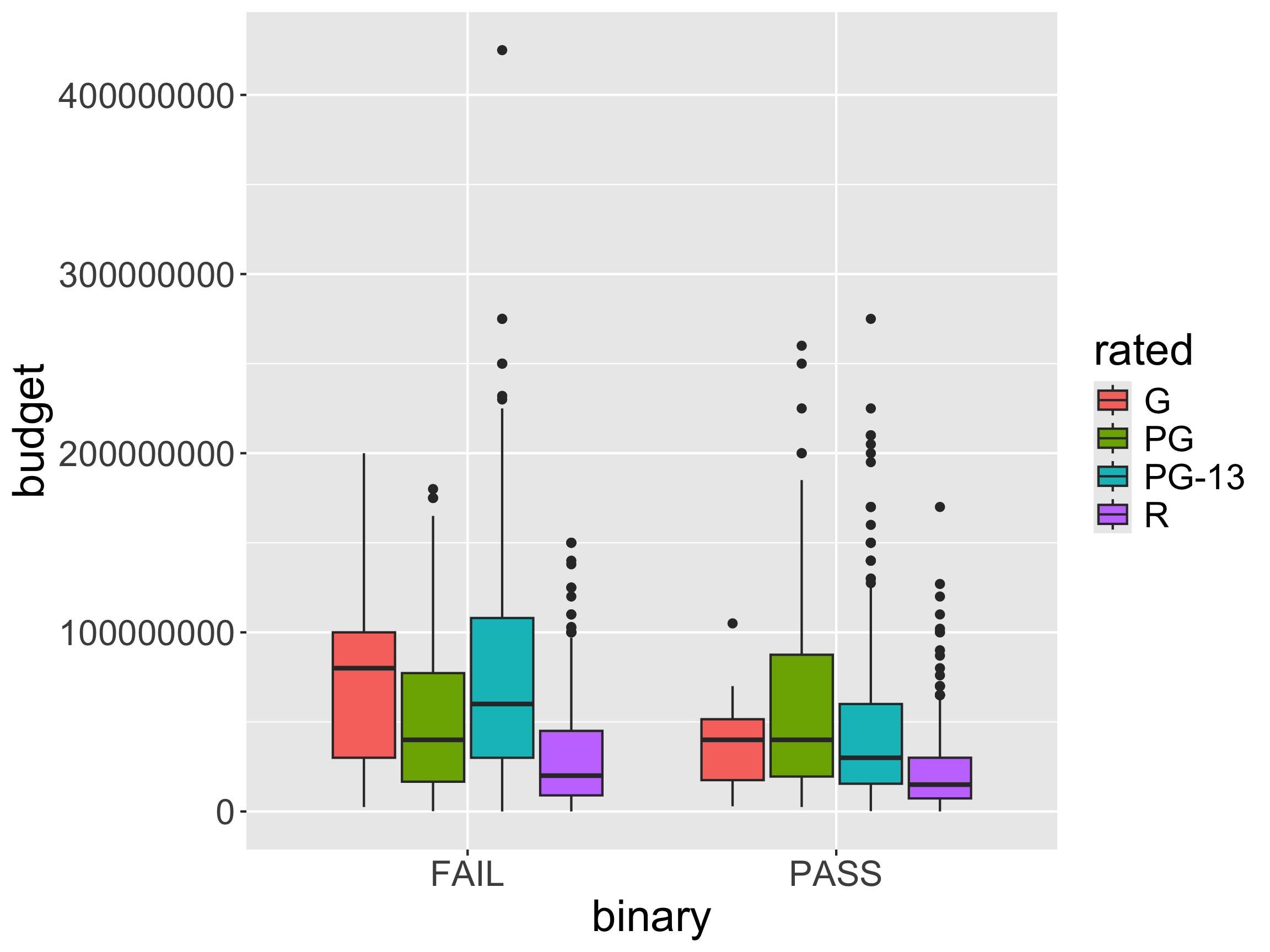
Distributions: geom_boxplot

Distributions: geom_boxplot
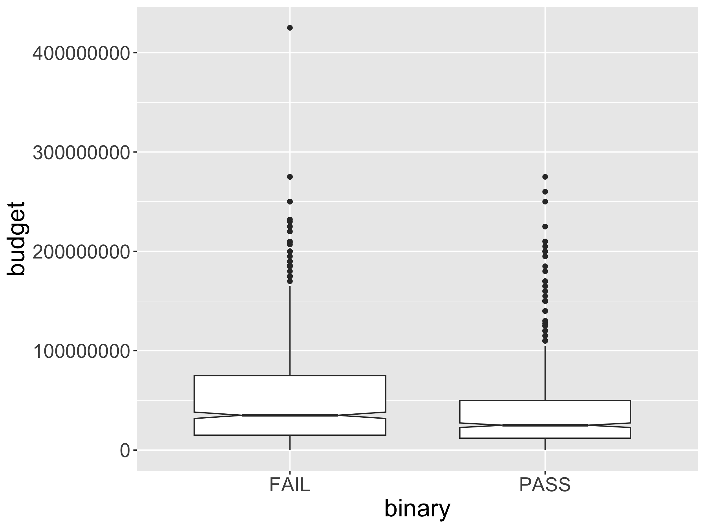
- What does
varwidthdo? - Why might we add
notch = TRUE?
Distributions: geom_boxplot
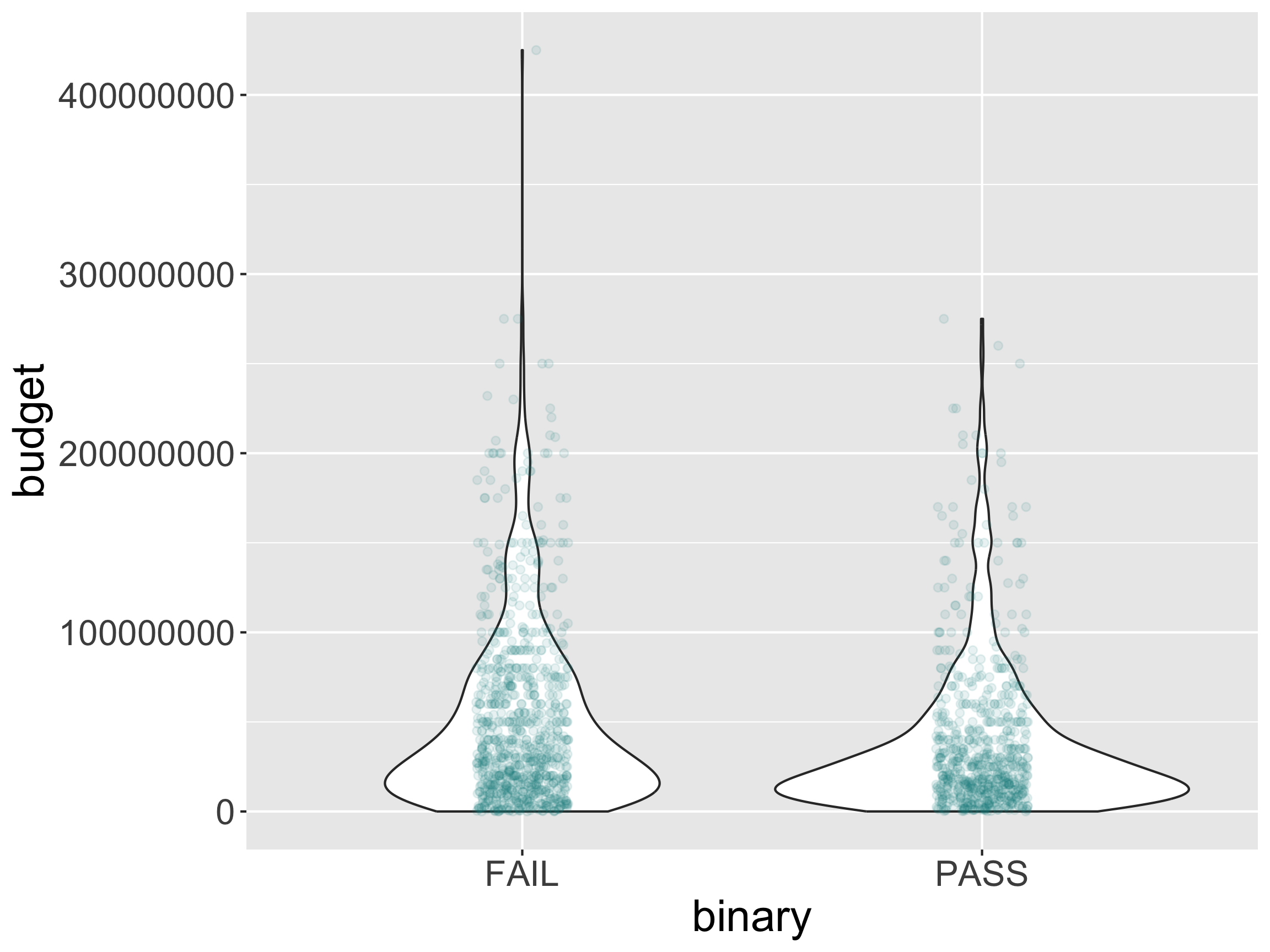
Distributions: geom_violin
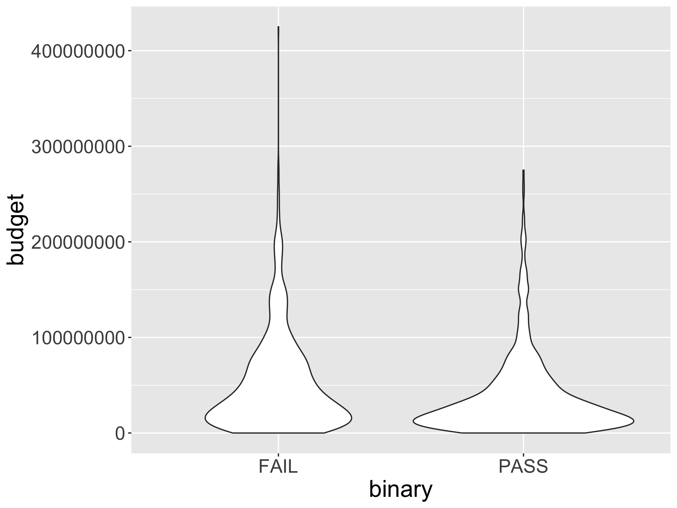
- Utility of the violin over the box?