Data Wrangling

Grayson White

Math 241
Week 3 | Spring 2026

Announcements

Office Hours Schedule
- Problem Set 1 due Thursday 9am.

Week 3 Goals

Mon Lecture

Think about reproducibility and learn how to ask coding questions well.
Motivate and work on data wrangling.

Wed Lecture

Plot animation and interactivity.
GitHub workflow review.

Reproducible Workflow

One where if you shared your data and work with someone else, they could reproduce your results.
Not the same as replication: Where someone collects new data following your same design to see if they get the same results.

Quarto documents allow us to include our R code, output, and narrative in the same place.
- Load the raw data.
- Be transparent about all the analysis steps.
- Even if you don’t showcase the R code in the output file, it is contained in the qmd file.

Creating `repr`oducible `ex`amples with `reprex`

Why do I need to learn to create reproducible technical examples?

So that you can ask and answer questions in our class Slack Workspace or Stack Overflow or other R help sites!

First, let’s take a look at some bad examples!

What is wrong with this coding question?

I am trying to create a plot and I can’t get the bars to do what I want them to. Help?!

What is wrong with this coding question?

I want to do the following but it isn’t working:

thing <- read.csv(“long/file/path/thing.csv”)

ggplot(thing, aes(x = factor(that))) + geom_bar()

Help?!

What is wrong with this coding question?

I want to reorder the bars of my plot but can’t get it working. Help!

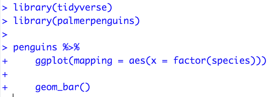
library(tidyverse)
library(palmerpenguins)

penguins <- penguins %>%
  group_by(species) %>%
  mutate(mean_flipper = mean(flipper_length_mm)) %>%
  ungroup() %>%
  mutate(long = case_when(flipper_length_mm < mean(flipper_length_mm) ~ "no",
                           flipper_length_mm >= mean(flipper_length_mm) ~ "yes"))  

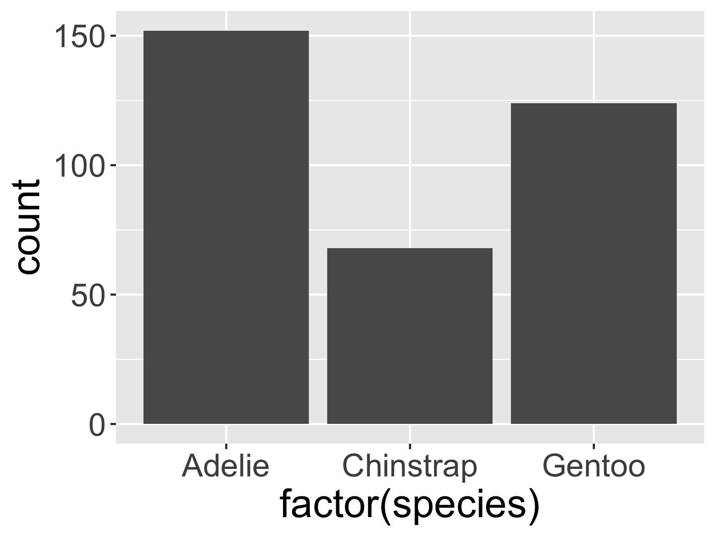
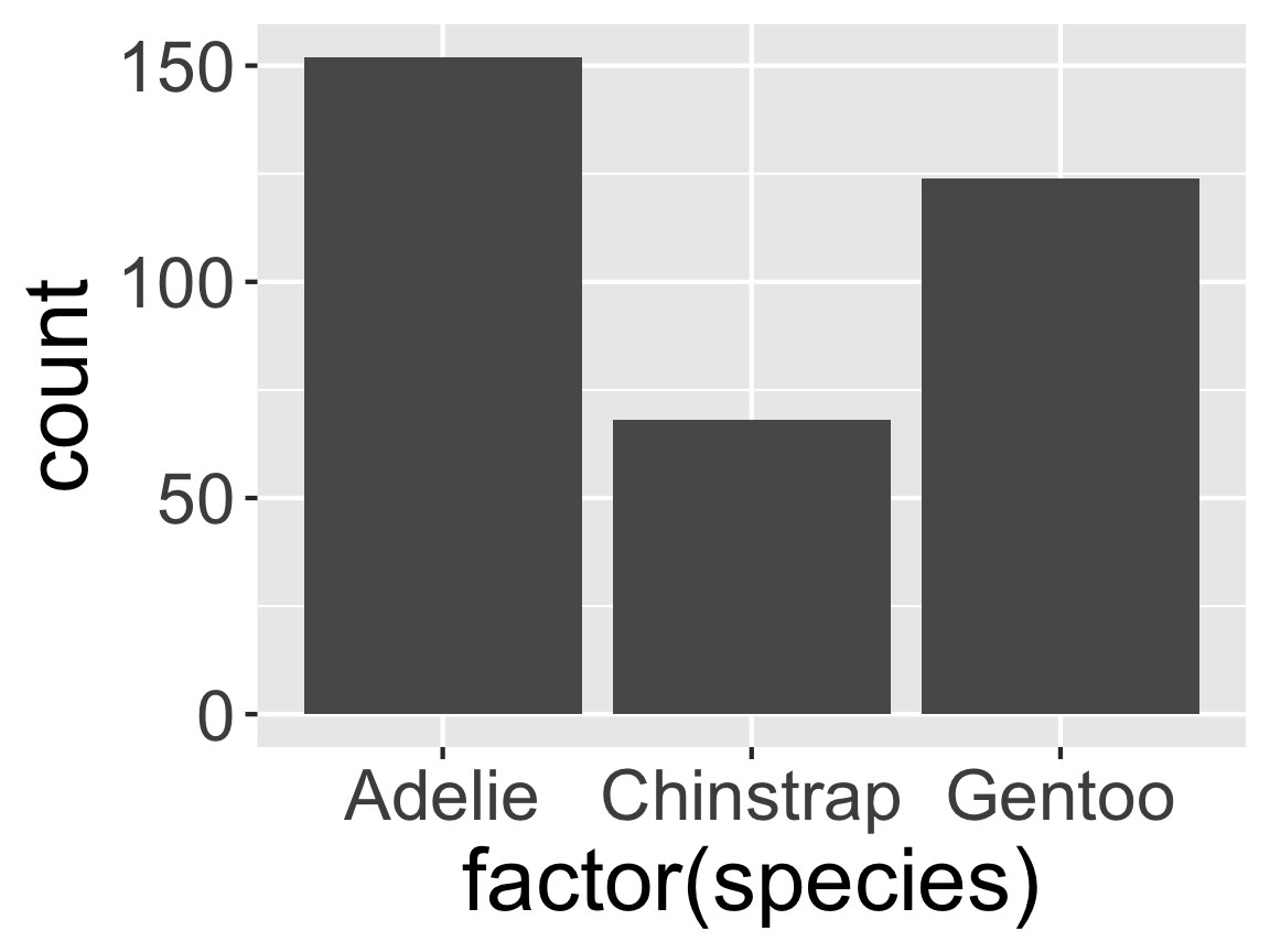
penguins %>%
  ggplot(mapping = aes(x = factor(species))) +
  geom_bar()

penguins %>%
  count(species)

What is wrong with this coding question?

I want to reorder the bars of my plot but can’t get it working. Help!

rm(list = ls())

library(tidyverse)
library(palmerpenguins)

penguins %>%
  ggplot(mapping = aes(x = factor(species))) +
  geom_bar()

What makes a good coding question?

It uses a minimal dataset to reproduce the issue.
It includes the shortest amount of runnable code necessary to reproduce the issue.
It doesn’t wreak havoc on other people’s computers.
It includes code and output so that others don’t have to run it!

It includes any necessary information on the used packages, R version, system, etc.
- Can use packageVersion("tidyverse") or sessionInfo() to find this information.

Minimal Dataset: two good options

Create a toy data frame.

dat <- data.frame(animal = c("cat", "dog", "mouse"), 
                  weight = c(5, 10, 0.5))
dat

  animal weight
1    cat    5.0
2    dog   10.0
3  mouse    0.5

Use a built-in dataset or a dataset from a particular package.

library(palmerpenguins)
penguins

# A tibble: 344 × 10
   species island    bill_length_mm bill_depth_mm flipper_length_mm body_mass_g
   <fct>   <fct>              <dbl>         <dbl>             <int>       <int>
 1 Adelie  Torgersen           39.1          18.7               181        3750
 2 Adelie  Torgersen           39.5          17.4               186        3800
 3 Adelie  Torgersen           40.3          18                 195        3250
 4 Adelie  Torgersen           NA            NA                  NA          NA
 5 Adelie  Torgersen           36.7          19.3               193        3450
 6 Adelie  Torgersen           39.3          20.6               190        3650
 7 Adelie  Torgersen           38.9          17.8               181        3625
 8 Adelie  Torgersen           39.2          19.6               195        4675
 9 Adelie  Torgersen           34.1          18.1               193        3475
10 Adelie  Torgersen           42            20.2               190        4250
# ℹ 334 more rows
# ℹ 4 more variables: sex <fct>, year <int>, mean_flipper <dbl>, long <chr>

Minimal Code

Include the necessary libraries.

Test run the code in a restarted R session to make sure it is runnable!

library(tidyverse)
library(palmerpenguins)

penguins %>%
  ggplot(mapping = aes(x = factor(species))) +
  geom_bar()

Make sure your code is copy-and-paste-able!

Don’t copy from the console.

> library(tidyverse)
> library(palmerpenguins)
> 
> penguins %>%
+     ggplot(mapping = aes(x = factor(species))) +
+     geom_bar()

Make sure your code is copy-and-paste-able!

Now we have our reproducible example:

How can I reorder the bars in the ggplot to go from the most frequent to the least frequent category?

library(tidyverse)
library(palmerpenguins)

penguins %>%
  ggplot(mapping = aes(x = factor(species))) +
  geom_bar()

How can we easily share it?

Using the reprex() function in the reprex package.

`reprex` Practice Time!

But first: Q: What is an R script file?

A text file for entering R commands.

Q: How is an R script file different from a Quarto or RMarkdown document?

You only put code in an R script.
If you add any text you must comment it out with #.
Think of it as a single R chunk that you won’t knit into an output document.
Useful when writing a lot of code and want to compartmentalize.

`reprex` Practice Time!

In Session, select “Clear Workspace” and then “Restart R”.
Open a script file and include in the top line:

library(reprex)

Put the code you want to use in the script file and make sure it runs.

library(tidyverse)
library(palmerpenguins)

penguins %>%
  ggplot(mapping = aes(x = factor(species))) +
  geom_bar()

Surround the code with reprex({ ... }, venue = "slack") and run it.
An md file will pop up. Copy all the contents of that file.
Head over to the #coding-qa channel and paste in the contents as a reply to the reprex practice message. A text box will pop-up and select “Apply”.
Above your code, type your question. Then hit “Send”.

Data Wrangling

So far, we’ve focused primarily on data visualization!

However, in order to make beautiful graphics, sometimes we have to go from

messy data ➡️ beautiful, wrangled, and cleaned data

Example: Data In the Wild

Many datasets on the internet are often in Display Format, not Analysis Format.

And, sometimes we’d like to modify a dataset to help us answer a specific question, or display the data in a particular way.
Many of you have already needed to do some data wrangling in Problem Set 1.

Recall this visualization from Week 1, Day 1

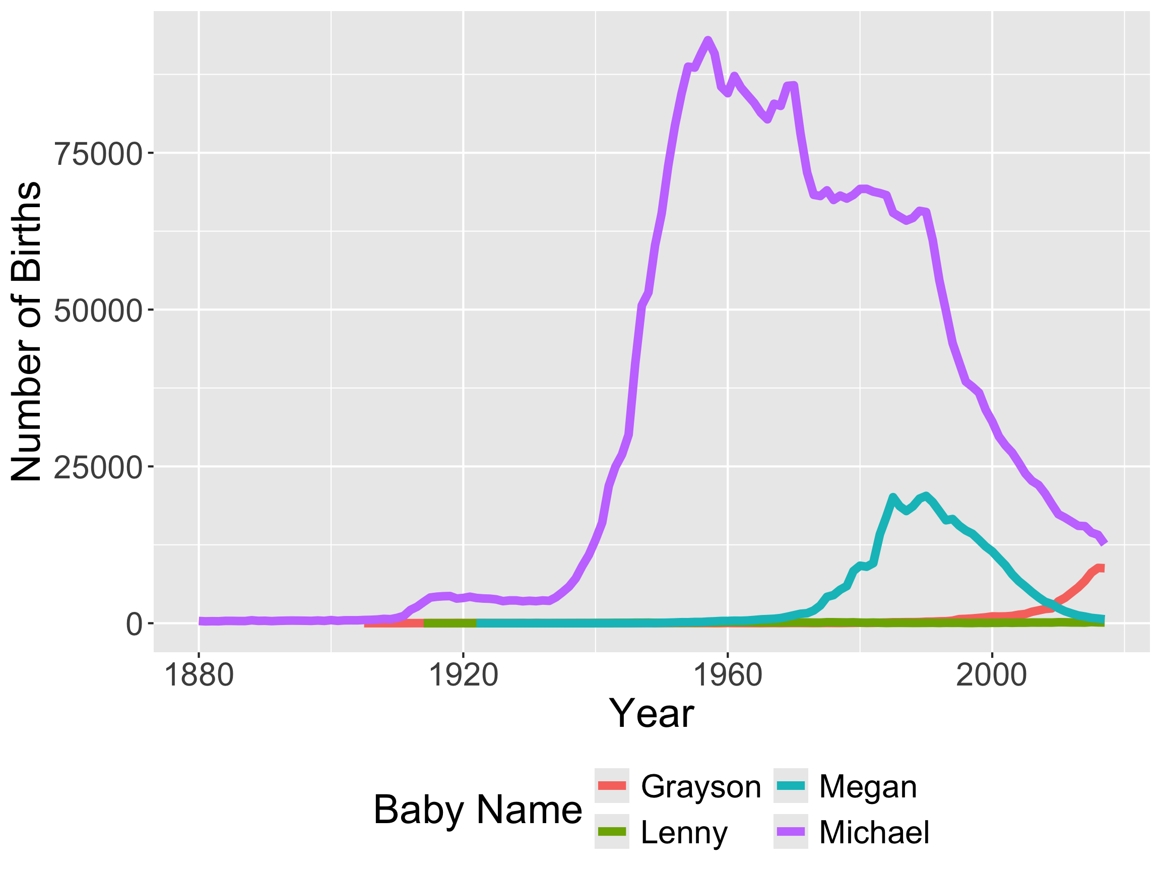
We need to be able to wrangle the data to make this visualization!

Recall this visualization from Week 1, Day 1

And to make the animated version!

In order to make these visualizations, we have to learn how to wrangle data!

Data Wrangling

What is it?
- Any processing you have to do to the data to summarize, visualize, model it.

Examples:
- Recoding 999 as “NA”
- Removing rows
- Creating new variables
- Recoding category variables
- Fixing variable types
- Reshaping data into a format that satisfies the tidy data principles

Data Wrangling

We are going to learn several packages to help us wrangle data.
We’ll learn the core of dplyr right now!

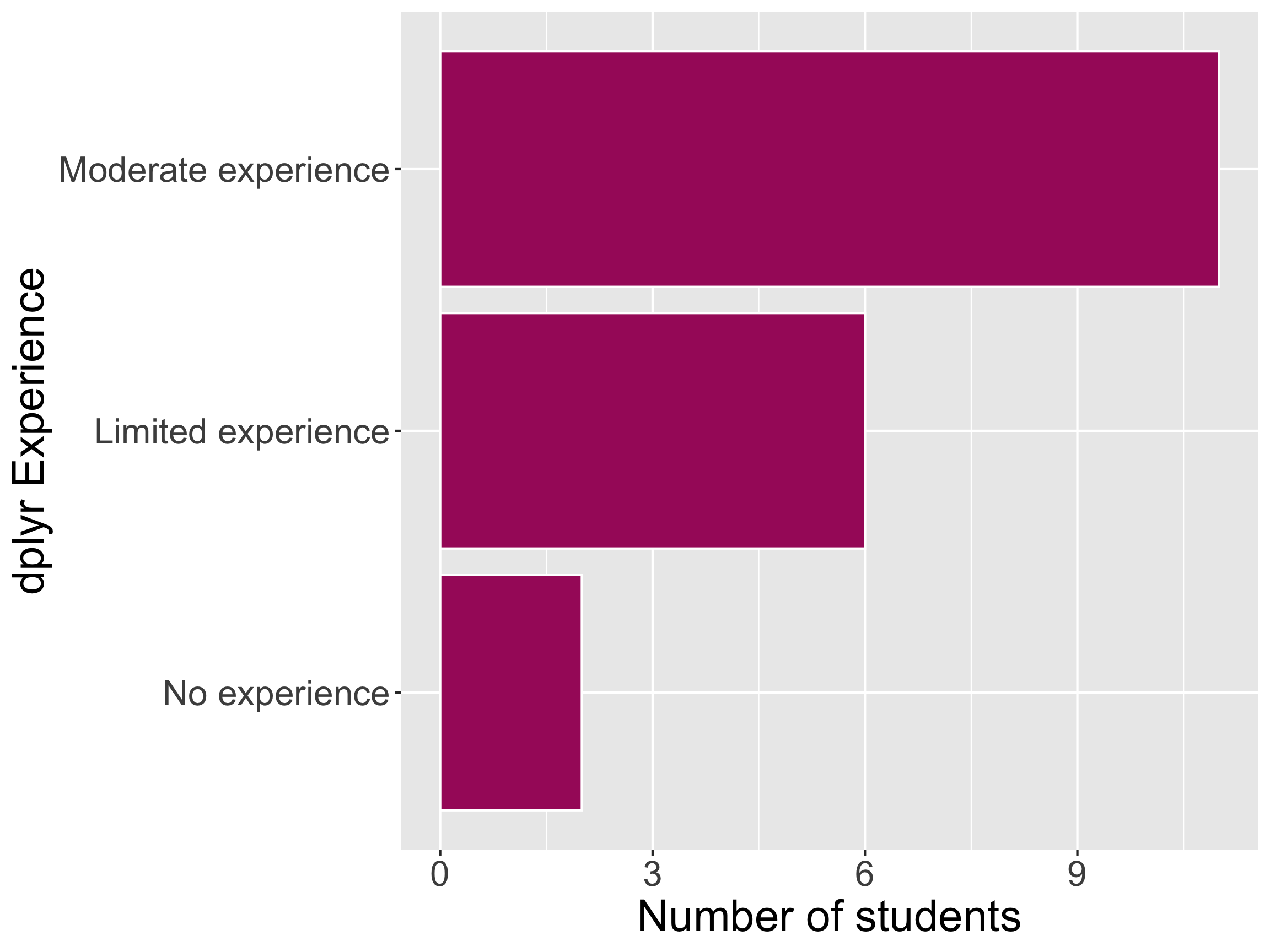
Math 241 `dplyr` Experience

`dplyr` core functions

dplyr for Data Wrangling

Common wrangling verbs:
- select()
- mutate()
- filter()
- arrange()
- summarize()
- drop_na()
- count()
One action:
- group_by()

Pipe for chaining together commands

magrittr pipe: %>%
New base R (native) pipe: |>
- Less flexible in some scenarios, but…
- Don’t need to load a package to use it

New data: `babynames`

library(babynames)
head(babynames)

# A tibble: 6 × 5
   year sex   name          n   prop
  <dbl> <chr> <chr>     <int>  <dbl>
1  1880 F     Mary       7065 0.0724
2  1880 F     Anna       2604 0.0267
3  1880 F     Emma       2003 0.0205
4  1880 F     Elizabeth  1939 0.0199
5  1880 F     Minnie     1746 0.0179
6  1880 F     Margaret   1578 0.0162

What does each row represent?

Wrangling `babynames`

What wrangling do we need to do to get from raw data to wrangled data?

library(babynames)
data("babynames")
head(babynames)

# A tibble: 6 × 5
   year sex   name          n   prop
  <dbl> <chr> <chr>     <int>  <dbl>
1  1880 F     Mary       7065 0.0724
2  1880 F     Anna       2604 0.0267
3  1880 F     Emma       2003 0.0205
4  1880 F     Elizabeth  1939 0.0199
5  1880 F     Minnie     1746 0.0179
6  1880 F     Margaret   1578 0.0162

head(babynames_math241)

# A tibble: 6 × 3
# Groups:   year [2]
   year name        n
  <dbl> <chr>   <int>
1  2017 Grayson  8767
2  2017 Lenny     118
3  2017 Megan     624
4  2017 Michael 12612
5  2016 Grayson  8817
6  2016 Lenny     134

Wrangling `babynames`

filter(): Subset rows based on logic statements.

babynames_math241 <- filter(babynames, 
                            name %in% c("Grayson", "Michael", 
                                        "Megan", "Lenny"))
babynames_math241

# A tibble: 675 × 5
    year sex   name        n    prop
   <dbl> <chr> <chr>   <int>   <dbl>
 1  1880 M     Michael   354 0.00299
 2  1881 M     Michael   298 0.00275
 3  1882 M     Michael   321 0.00263
 4  1883 M     Michael   307 0.00273
 5  1884 M     Michael   373 0.00304
 6  1885 M     Michael   370 0.00319
 7  1886 M     Michael   348 0.00292
 8  1887 M     Michael   345 0.00316
 9  1888 M     Michael   466 0.00359
10  1889 M     Michael   377 0.00317
# ℹ 665 more rows

Wrangling `babynames`

%>% (the pipe): Inserts current line as first argument in the next line.

babynames_math241 <- filter(babynames, 
                            name %in% c("Grayson", "Michael",
                                        "Megan", "Lenny"))

babynames_math241

# A tibble: 675 × 5
    year sex   name        n    prop
   <dbl> <chr> <chr>   <int>   <dbl>
 1  1880 M     Michael   354 0.00299
 2  1881 M     Michael   298 0.00275
 3  1882 M     Michael   321 0.00263
 4  1883 M     Michael   307 0.00273
 5  1884 M     Michael   373 0.00304
 6  1885 M     Michael   370 0.00319
 7  1886 M     Michael   348 0.00292
 8  1887 M     Michael   345 0.00316
 9  1888 M     Michael   466 0.00359
10  1889 M     Michael   377 0.00317
# ℹ 665 more rows

Wrangling `babynames`

%>% (the pipe): Inserts current line as first argument in the next line.

babynames_math241 <- filter(babynames, 
                            name %in% c("Grayson", "Michael",
                                        "Megan", "Lenny"))

# this operation does exactly the same thing as above
babynames_math241 <- babynames %>%
  filter(name %in% c("Grayson", "Michael",
                     "Megan", "Lenny"))

babynames_math241

# A tibble: 675 × 5
    year sex   name        n    prop
   <dbl> <chr> <chr>   <int>   <dbl>
 1  1880 M     Michael   354 0.00299
 2  1881 M     Michael   298 0.00275
 3  1882 M     Michael   321 0.00263
 4  1883 M     Michael   307 0.00273
 5  1884 M     Michael   373 0.00304
 6  1885 M     Michael   370 0.00319
 7  1886 M     Michael   348 0.00292
 8  1887 M     Michael   345 0.00316
 9  1888 M     Michael   466 0.00359
10  1889 M     Michael   377 0.00317
# ℹ 665 more rows

Wrangling `babynames`

summarize(): Compute an aggregation measure (e.g., mean, standard deviation).

babynames_math241 <- babynames %>%
  filter(name %in% c("Grayson", "Michael",
                     "Megan", "Lenny")) %>%
  summarize(n = sum(n))

babynames_math241

# A tibble: 1 × 1
        n
    <int>
1 4892634

Wrangling `babynames`

group_by(): Create groups for how future operations should be computed.

babynames_math241 <- babynames %>%
  filter(name %in% c("Grayson", "Michael",
                     "Megan", "Lenny")) %>%
  group_by(name) %>%
  summarize(n = sum(n))

babynames_math241

# A tibble: 4 × 2
  name          n
  <chr>     <int>
1 Grayson   74707
2 Lenny      7768
3 Megan    437623
4 Michael 4372536

What are we missing?

Wrangling `babynames`

group_by(): Create groups for how future operations should be computed.

babynames_math241 <- babynames %>%
  filter(name %in% c("Grayson", "Michael",
                     "Megan", "Lenny")) %>%
  group_by(year, name) %>%
  summarize(n = sum(n)) 

babynames_math241

# A tibble: 431 × 3
# Groups:   year [138]
    year name        n
   <dbl> <chr>   <int>
 1  1880 Michael   354
 2  1881 Michael   298
 3  1882 Michael   321
 4  1883 Michael   307
 5  1884 Michael   373
 6  1885 Michael   370
 7  1886 Michael   348
 8  1887 Michael   345
 9  1888 Michael   466
10  1889 Michael   377
# ℹ 421 more rows

Wrangling `babynames`

group_by(): Create groups for how future operations should be computed.

babynames_math241 <- babynames %>%
  filter(name %in% c("Grayson", "Michael",
                     "Megan", "Lenny")) %>%
  group_by(year, name) %>%
  summarize(n = sum(n)) %>%
  ungroup()

babynames_math241

# A tibble: 431 × 3
    year name        n
   <dbl> <chr>   <int>
 1  1880 Michael   354
 2  1881 Michael   298
 3  1882 Michael   321
 4  1883 Michael   307
 5  1884 Michael   373
 6  1885 Michael   370
 7  1886 Michael   348
 8  1887 Michael   345
 9  1888 Michael   466
10  1889 Michael   377
# ℹ 421 more rows

What did ungroup() do?

Wrangling `babynames`

arrange(): Order the rows by variable(s).

babynames_math241 <- babynames %>%
  filter(name %in% c("Grayson", "Michael",
                     "Megan", "Lenny")) %>%
  group_by(year, name) %>%
  summarize(n = sum(n)) %>%
  ungroup() %>%
  arrange(desc(year))

babynames_math241

# A tibble: 431 × 3
    year name        n
   <dbl> <chr>   <int>
 1  2017 Grayson  8767
 2  2017 Lenny     118
 3  2017 Megan     624
 4  2017 Michael 12612
 5  2016 Grayson  8817
 6  2016 Lenny     134
 7  2016 Megan     744
 8  2016 Michael 14091
 9  2015 Grayson  8071
10  2015 Lenny     177
# ℹ 421 more rows

New data: pets I’ve had

my_pets <- data.frame(
  name = c("Dude", "Pickle", "Kyle", "Nubs"),
  type = c("dog", "cat", "cat", "cat"),
  age = c(8, 6, 4, NA),
  birthplace = c("Washington", NA, "Utah", NA)
)

my_pets

    name type age birthplace
1   Dude  dog   8 Washington
2 Pickle  cat   6       <NA>
3   Kyle  cat   4       Utah
4   Nubs  cat  NA       <NA>

Wrangling `my_pets`

select(): retain particular columns.

my_pets %>%
  select(name, type, age)

    name type age
1   Dude  dog   8
2 Pickle  cat   6
3   Kyle  cat   4
4   Nubs  cat  NA

Wrangling `my_pets`

select(): retain particular columns.

my_pets %>%
  select(-birthplace)

    name type age
1   Dude  dog   8
2 Pickle  cat   6
3   Kyle  cat   4
4   Nubs  cat  NA

Wrangling `my_pets`

drop_na(): Remove any row that has a missing value for particular variables.

my_pets %>%
  drop_na(birthplace)

  name type age birthplace
1 Dude  dog   8 Washington
2 Kyle  cat   4       Utah

Wrangling `my_pets`

mutate(): Create new variables or modify existing variables

Use case: pet years!
- 8 for large dog, 7 for cats
- (I’m not an animal scientist)

my_pets <- my_pets %>%
  # bad solution
  mutate(age_pet_years = age * 7.5)

my_pets

    name type age birthplace age_pet_years
1   Dude  dog   8 Washington            60
2 Pickle  cat   6       <NA>            45
3   Kyle  cat   4       Utah            30
4   Nubs  cat  NA       <NA>            NA

Wrangling `my_pets`

mutate(): Create new variables or modify existing variables

Use case: pet years!
- 8 for large dog, 7 for cats
- (I’m not an animal scientist)

Better solution: use case_when()

my_pets <- my_pets %>%
  mutate(age_pet_years = case_when(
    type == "dog" ~ 8 * age,
    type == "cat" ~ 7 * age
    ))

my_pets

    name type age birthplace age_pet_years
1   Dude  dog   8 Washington            64
2 Pickle  cat   6       <NA>            42
3   Kyle  cat   4       Utah            28
4   Nubs  cat  NA       <NA>            NA

Wrangling `my_pets`

More filter()ing

pets_who_can_drink <- my_pets %>%
  filter(age_pet_years > 21)

pets_who_can_drink

    name type age birthplace age_pet_years
1   Dude  dog   8 Washington            64
2 Pickle  cat   6       <NA>            42
3   Kyle  cat   4       Utah            28

Wrangling `my_pets`

More filter()ing: Nubs seemed like he was pretty old

pets_who_can_drink <- my_pets %>%
  filter(age_pet_years > 21 & is.na(age_pet_years))

pets_who_can_drink

[1] name          type          age           birthplace    age_pet_years
<0 rows> (or 0-length row.names)

What went wrong here???
Logical operators: & means ‘and’

Wrangling `my_pets`

More filter()ing: Nubs seemed like he was pretty old

pets_who_can_drink <- my_pets %>%
  filter(age_pet_years > 21 | is.na(age_pet_years))

pets_who_can_drink

    name type age birthplace age_pet_years
1   Dude  dog   8 Washington            64
2 Pickle  cat   6       <NA>            42
3   Kyle  cat   4       Utah            28
4   Nubs  cat  NA       <NA>            NA

Logical operators: | means ‘or’

Wrangling `my_pets`

More filter()ing

old_cats <- my_pets %>%
  filter(age_pet_years > 30, type == "dog")

old_cats

  name type age birthplace age_pet_years
1 Dude  dog   8 Washington            64

In a filter(), the comma implicitly means &

Wrangling `my_pets`

%in% vs. ==

my_pets %>%
  filter(name == c("Dude", "Kyle"))

  name type age birthplace age_pet_years
1 Dude  dog   8 Washington            64

What went wrong here?

Wrangling `my_pets`

%in% vs. ==

my_pets %>%
  filter(name %in% c("Dude", "Kyle"))

  name type age birthplace age_pet_years
1 Dude  dog   8 Washington            64
2 Kyle  cat   4       Utah            28

Activity

15:00

Next time

Use some of our data wrangling skills to make animated and interactive graphics!

Announcements

Week 3 Goals

Reproducible Workflow

Creating reproducible examples with reprex

Why do I need to learn to create reproducible technical examples?

First, let’s take a look at some bad examples!

What is wrong with this coding question?

What is wrong with this coding question?

What is wrong with this coding question?

What is wrong with this coding question?

What makes a good coding question?

Minimal Dataset: two good options

Minimal Code

Make sure your code is copy-and-paste-able!

Make sure your code is copy-and-paste-able!

Now we have our reproducible example:

reprex Practice Time!

reprex Practice Time!

Data Wrangling

Data Wrangling

Example: Data In the Wild

Recall this visualization from Week 1, Day 1

Recall this visualization from Week 1, Day 1

Data Wrangling

Data Wrangling

Math 241 dplyr Experience

dplyr core functions

dplyr for Data Wrangling

Pipe for chaining together commands

New data: babynames

Wrangling babynames

What wrangling do we need to do to get from raw data to wrangled data?

Wrangling babynames

Wrangling babynames

Wrangling babynames

Wrangling babynames

Wrangling babynames

Wrangling babynames

Wrangling babynames

Wrangling babynames

New data: pets I’ve had

Wrangling my_pets

Wrangling my_pets

Wrangling my_pets

Wrangling my_pets

Wrangling my_pets

Wrangling my_pets

Wrangling my_pets

Wrangling my_pets

Wrangling my_pets

Wrangling my_pets

Wrangling my_pets

Activity

Next time

Creating `repr`oducible `ex`amples with `reprex`

`reprex` Practice Time!

`reprex` Practice Time!

Math 241 `dplyr` Experience

`dplyr` core functions

New data: `babynames`

Wrangling `babynames`

Wrangling `babynames`

Wrangling `babynames`

Wrangling `babynames`

Wrangling `babynames`

Wrangling `babynames`

Wrangling `babynames`

Wrangling `babynames`

Wrangling `babynames`

Wrangling `my_pets`

Wrangling `my_pets`

Wrangling `my_pets`

Wrangling `my_pets`

Wrangling `my_pets`

Wrangling `my_pets`

Wrangling `my_pets`

Wrangling `my_pets`

Wrangling `my_pets`

Wrangling `my_pets`

Wrangling `my_pets`