Data Wrangling and Types

Grayson White

Math 241
Week 4 | Spring 2026

Announcements

Welcome to the newly admitted students!
Office hours time change going forward.

Course Interest Form

04:00

Week 4 Goals

Mon Lecture

Different types of data in R
- atomic and generic vectors
- subsetting objects
Talk more about logical statements
More practice with dplyr verbs and data wrangling

Wed Lecture

Joining multiple data frames
“Tidy” data
Reshaping data frames

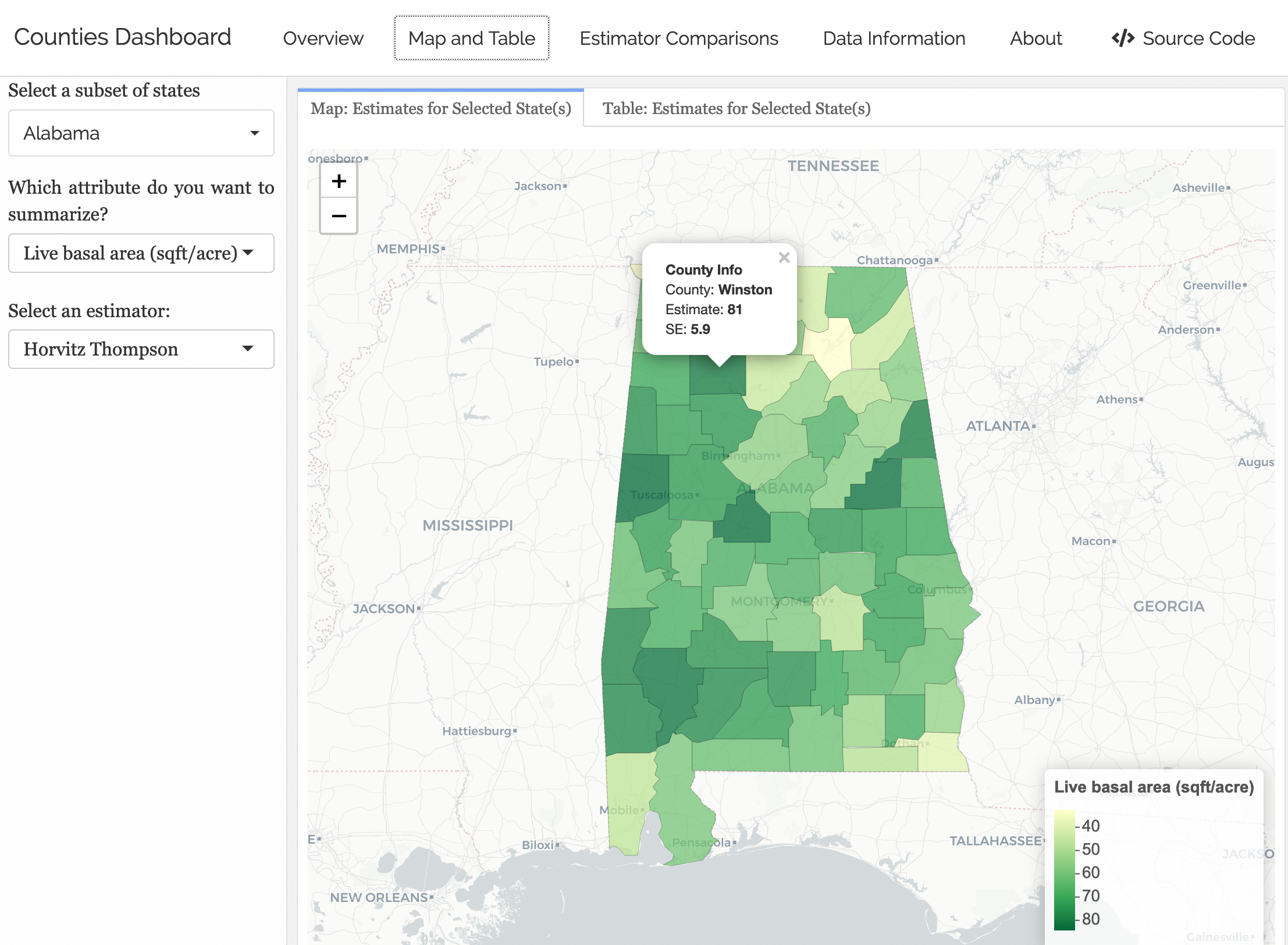
Looking Ahead to Project 1

Goal: Create interactive dashboards with shinydashboard and flexdashboard.

Link to example dashboard

What We Need First

Need a robust understanding of wrangling data frames.
Need to explore more data objects in R.
Need to learn how to interact with and wrangle these data objects.

`dplyr` review

Data: Census 2000 (from `openintro`)

library(openintro)
data(census)
census %>% head(n = 5)

# A tibble: 5 × 8
  census_year state_fips_code total_family_income   age sex    race_general   
        <int> <fct>                         <int> <int> <fct>  <fct>          
1        2000 Florida                       14550    44 Male   Two major races
2        2000 Florida                       22800    20 Female White          
3        2000 Florida                           0    20 Male   Black          
4        2000 Florida                       23000     6 Female White          
5        2000 Florida                       48000    55 Male   White          
# ℹ 2 more variables: marital_status <fct>, total_personal_income <int>

`select()`

Use select() to grab only the variables/columns we want

census %>%
  select(census_year, age, sex, marital_status)

# A tibble: 500 × 4
   census_year   age sex    marital_status        
         <int> <int> <fct>  <fct>                 
 1        2000    44 Male   Married/spouse present
 2        2000    20 Female Never married/single  
 3        2000    20 Male   Never married/single  
 4        2000     6 Female Never married/single  
 5        2000    55 Male   Married/spouse present
 6        2000    43 Female Married/spouse present
 7        2000    60 Female Married/spouse present
 8        2000    47 Female Married/spouse present
 9        2000    54 Female Married/spouse present
10        2000    58 Female Widowed               
# ℹ 490 more rows

`select()`

Or you can add minus signs to delete columns from the dataset.

census %>%
  select(-census_year, -age, -sex, -marital_status)

# A tibble: 500 × 4
   state_fips_code total_family_income race_general    total_personal_income
   <fct>                         <int> <fct>                           <int>
 1 Florida                       14550 Two major races                     0
 2 Florida                       22800 White                           13000
 3 Florida                           0 Black                           20000
 4 Florida                       23000 White                              NA
 5 Florida                       48000 White                           36000
 6 Florida                       74000 White                           27000
 7 Florida                       23000 White                           11800
 8 Florida                       74000 White                           48000
 9 Florida                       60000 Black                           40000
10 Florida                       14600 White                           14600
# ℹ 490 more rows

`mutate()`

mutate() can add new columns that are functions of existing columns:

census %>%
  mutate(age_decade = (age %/% 10)) %>%
  select(census_year, state_fips_code, total_family_income, age, age_decade)

# A tibble: 500 × 5
   census_year state_fips_code total_family_income   age age_decade
         <int> <fct>                         <int> <int>      <dbl>
 1        2000 Florida                       14550    44          4
 2        2000 Florida                       22800    20          2
 3        2000 Florida                           0    20          2
 4        2000 Florida                       23000     6          0
 5        2000 Florida                       48000    55          5
 6        2000 Florida                       74000    43          4
 7        2000 Florida                       23000    60          6
 8        2000 Florida                       74000    47          4
 9        2000 Florida                       60000    54          5
10        2000 Florida                       14600    58          5
# ℹ 490 more rows

New operator: %/% does integer division

`filter()`

filter() only keeps rows/observations that match certain criteria

census %>%
  filter(age < 25, sex == 'Female')

# A tibble: 80 × 8
   census_year state_fips_code total_family_income   age sex    race_general
         <int> <fct>                         <int> <int> <fct>  <fct>       
 1        2000 Florida                       22800    20 Female White       
 2        2000 Florida                       23000     6 Female White       
 3        2000 Florida                      103700     8 Female White       
 4        2000 Florida                       70700    17 Female White       
 5        2000 Florida                      118100    18 Female White       
 6        2000 New York                      68020     2 Female Chinese     
 7        2000 New York                      50400    21 Female White       
 8        2000 New York                      65000     1 Female White       
 9        2000 New York                      62900    17 Female Black       
10        2000 New York                     168200     6 Female White       
# ℹ 70 more rows
# ℹ 2 more variables: marital_status <fct>, total_personal_income <int>

`arrange()`

arrange() sorts the rows by a certain variable (or set of variables)

census %>%
  arrange(age)

# A tibble: 500 × 8
   census_year state_fips_code total_family_income   age sex    race_general   
         <int> <fct>                         <int> <int> <fct>  <fct>          
 1        2000 Texas                          9200     0 Male   Black          
 2        2000 Florida                       48000     1 Male   White          
 3        2000 New York                      13000     1 Male   White          
 4        2000 New York                      65000     1 Female White          
 5        2000 Michigan                      57400     1 Female White          
 6        2000 Pennsylvania                  27150     1 Male   White          
 7        2000 Florida                       50090     2 Male   White          
 8        2000 Florida                        6000     2 Male   White          
 9        2000 New York                      68020     2 Female Chinese        
10        2000 New York                      17000     2 Male   Two major races
# ℹ 490 more rows
# ℹ 2 more variables: marital_status <fct>, total_personal_income <int>

`arrange()`

Can do descending order too with the desc() function!

census %>%
  arrange(desc(age))

# A tibble: 500 × 8
   census_year state_fips_code total_family_income   age sex    race_general
         <int> <fct>                         <int> <int> <fct>  <fct>       
 1        2000 Louisiana                      8100    93 Female White       
 2        2000 Illinois                         NA    87 Female White       
 3        2000 West Virginia                     0    87 Male   White       
 4        2000 Delaware                      46200    85 Female White       
 5        2000 Indiana                        8000    85 Male   Black       
 6        2000 New York                      15570    83 Male   White       
 7        2000 New York                       8800    82 Female White       
 8        2000 Massachusetts                 34300    82 Female White       
 9        2000 New York                      55000    81 Male   White       
10        2000 Minnesota                         0    81 Female White       
# ℹ 490 more rows
# ℹ 2 more variables: marital_status <fct>, total_personal_income <int>

`arrange()`

Can arrange by multiple variables too:

census %>%
  arrange(age, sex)

# A tibble: 500 × 8
   census_year state_fips_code total_family_income   age sex    race_general
         <int> <fct>                         <int> <int> <fct>  <fct>       
 1        2000 Texas                          9200     0 Male   Black       
 2        2000 New York                      65000     1 Female White       
 3        2000 Michigan                      57400     1 Female White       
 4        2000 Florida                       48000     1 Male   White       
 5        2000 New York                      13000     1 Male   White       
 6        2000 Pennsylvania                  27150     1 Male   White       
 7        2000 New York                      68020     2 Female Chinese     
 8        2000 Maryland                      95500     2 Female White       
 9        2000 Oregon                         9300     2 Female White       
10        2000 Michigan                      20340     2 Female White       
# ℹ 490 more rows
# ℹ 2 more variables: marital_status <fct>, total_personal_income <int>

`summarize()`

summarize() computes summary statistics and collapses data into row(s) that show those summary statistics

census %>%
  summarize(mean_income = mean(total_family_income, na.rm = TRUE),
            sd_income = sd(total_family_income, na.rm = TRUE),
            size = n())

# A tibble: 1 × 3
  mean_income sd_income  size
        <dbl>     <dbl> <int>
1      57411.    70732.   500

Can compute multiple measures

`group_by()` + `summarize()`

Add group_by() to summarize() to calculate summary statistics by specified grouping variable(s)

census %>%
  group_by(state_fips_code) %>%
  summarize(mean_income = mean(total_family_income, na.rm = TRUE),
            sd_income = sd(total_family_income, na.rm = TRUE),
            size = n()) %>%
  filter(size > 10) %>%
  arrange(mean_income)

# A tibble: 14 × 4
   state_fips_code mean_income sd_income  size
   <fct>                 <dbl>     <dbl> <int>
 1 Washington           20079.    12980.    11
 2 Louisiana            34899.    42097.    12
 3 Ohio                 40748.    26796.    23
 4 Indiana              46738.    32291.    17
 5 Florida              46848.    31787.    39
 6 Pennsylvania         51685     44823.    26
 7 Illinois             55972.    42426.    21
 8 New York             57064.    44793.    43
 9 Texas                58240.    72468.    37
10 Michigan             59160     27403.    14
11 Massachusetts        59506.    38984.    12
12 Georgia              60488.    52199.    18
13 California           73142.    69338.    62
14 New Jersey           77498     80288.    15

Tip: `count()`

count() is a short-cut for group_by() + summarize(n())

census %>% 
  group_by(sex) %>%
  summarize(n())

# A tibble: 2 × 2
  sex    `n()`
  <fct>  <int>
1 Female   232
2 Male     268

census %>% count(sex)

# A tibble: 2 × 2
  sex        n
  <fct>  <int>
1 Female   232
2 Male     268

`group_by()` + `mutate()`

Adding group_by() allows functions (e.g., sum()) to operate on variables by specified grouping variable(s)

Let’s start with this summary dataset:

temp <- census %>%
  count(marital_status, sex)
temp

# A tibble: 12 × 3
   marital_status         sex        n
   <fct>                  <fct>  <int>
 1 Divorced               Female    21
 2 Divorced               Male      17
 3 Married/spouse absent  Female     5
 4 Married/spouse absent  Male       9
 5 Married/spouse present Female    92
 6 Married/spouse present Male     100
 7 Never married/single   Female    93
 8 Never married/single   Male     129
 9 Separated              Female     1
10 Separated              Male       2
11 Widowed                Female    20
12 Widowed                Male      11

`group_by()` + `mutate()`

temp %>%
  mutate(p = n / sum(n))

# A tibble: 12 × 4
   marital_status         sex        n     p
   <fct>                  <fct>  <int> <dbl>
 1 Divorced               Female    21 0.042
 2 Divorced               Male      17 0.034
 3 Married/spouse absent  Female     5 0.01 
 4 Married/spouse absent  Male       9 0.018
 5 Married/spouse present Female    92 0.184
 6 Married/spouse present Male     100 0.2  
 7 Never married/single   Female    93 0.186
 8 Never married/single   Male     129 0.258
 9 Separated              Female     1 0.002
10 Separated              Male       2 0.004
11 Widowed                Female    20 0.04 
12 Widowed                Male      11 0.022

Q: What is the denominator for the proportions in the new p variable?

`group_by()` + `mutate()`

temp %>%
  group_by(marital_status) %>% # added this!
  mutate(p = n / sum(n))

# A tibble: 12 × 4
# Groups:   marital_status [6]
   marital_status         sex        n     p
   <fct>                  <fct>  <int> <dbl>
 1 Divorced               Female    21 0.553
 2 Divorced               Male      17 0.447
 3 Married/spouse absent  Female     5 0.357
 4 Married/spouse absent  Male       9 0.643
 5 Married/spouse present Female    92 0.479
 6 Married/spouse present Male     100 0.521
 7 Never married/single   Female    93 0.419
 8 Never married/single   Male     129 0.581
 9 Separated              Female     1 0.333
10 Separated              Male       2 0.667
11 Widowed                Female    20 0.645
12 Widowed                Male      11 0.355

Q: Now what is the denominator for the proportions in the new p variable?

Now: type of data objects

Math 241 `R` Data Objects So Far:

Data frames:

crash_data <- read_csv("data/pdx_crash_2018_page1.csv") 
class(crash_data)

[1] "spec_tbl_df" "tbl_df"      "tbl"         "data.frame"

(Atomic) Vectors:

pretty_colors <- c("steelblue", "seagreen", "goldenrod")
class(pretty_colors)

[1] "character"

size <- 3
class(size)

[1] "numeric"

The last two are both examples of what are called atomic vectors.

R Objects: Vectors

Vectors are the fundamental building blocks of data in R.
- Each column in a data frame is an atomic vector!
- Come in 2 flavors!

Flavor 1: Atomic vectors
- Homogeneous collections of the same type.
- Confusingly, people usually just call these vectors.

Flavor 2: Generic vectors
- Heterogeneous collections of any type of R objects.
- Commonly called lists.

Deep Dive into (atomic) vectors

Let’s explore the common types and how to interact with them.
This will allow us to use vectors to do useful things,
Understand logical statements and dplyr more robustly, and
debug our code more effectively!

Flavors of Atomic Vectors

Logical: TRUEs and FALSEs

happy <- c(TRUE, FALSE, TRUE, TRUE)
class(happy)

[1] "logical"

Numeric: Integers, real numbers (double-precision floating point numbers)

x <- c(1, 4, 5)
class(x)

[1] "numeric"

x <- c(1L, 4L, 5L)
class(x)

[1] "integer"

Character: Strings (contains 1 or more characters)

animals <- c("mountain goat", "lemur", "capybara")
class(animals)

[1] "character"

Factors: Strings with order

animals <- as.factor(animals)
class(animals)

[1] "factor"

Factors versus Characters

Character: Strings (contains 1 or more characters)

animals <- c("mountain goat", "lemur", "capybara")
class(animals)

[1] "character"

typeof(animals)

[1] "character"

str(animals)

 chr [1:3] "mountain goat" "lemur" "capybara"

Factors: Strings with order

animals <- as.factor(animals)
class(animals)

[1] "factor"

typeof(animals)

[1] "integer"

str(animals)

 Factor w/ 3 levels "capybara","lemur",..: 3 2 1

What?!

If you want to read more about this rabbit hole, go here.

Concatenation

Atomic vectors are created and combined with c().

x <- 5
x

[1] 5

y <- c(4, 1, 7)
y

[1] 4 1 7

z <- c(y, x, c(20))
z

[1]  4  1  7  5 20

quick <- c(2:5, 13)
quick

[1]  2  3  4  5 13

Checking Type

is.logical(c(FALSE, TRUE))

[1] TRUE

is.logical(c(0, 1))

[1] FALSE

is.factor(c("mountain goat", "lemur", "capybara"))

[1] FALSE

is.character(c("mountain goat", "lemur", "capybara"))

[1] TRUE

Checking Type

is.integer(1)

[1] FALSE

is.double(1)

[1] TRUE

is.numeric(1)

[1] TRUE

is.atomic(1)

[1] TRUE

is.integer(1L)

[1] TRUE

is.double(1L)

[1] FALSE

is.numeric(1L)

[1] TRUE

is.atomic(1L)

[1] TRUE

Type Coercion

R will often change the type of a vector with no warning.
Usually it makes the smart choice.

y <- c(4, 1, 7)
class(y)

[1] "numeric"

z <- c(y, "cat")
class(z)

[1] "character"

[1] "4"   "1"   "7"   "cat"

z <- c(y, 3L)
class(z)

[1] "numeric"

[1] 4 1 7 3

a <- c(FALSE, 4)
class(a)

[1] "numeric"

[1] 0 4

b <- c(NA, 4)
class(b)

[1] "numeric"

[1] NA  4

Operator Coercion

Functions and operators (like +, -, *, etc.) will often try to convert a vector to an appropriate type.
Once we are writing our own functions, we will consider building in tests to ensure the user provided the correct type.

1L + 3.1415

[1] 4.1415

log(TRUE)

[1] 0

sum(c(FALSE, TRUE, TRUE))

[1] 2

TRUE & FALSE

[1] FALSE

TRUE | FALSE

[1] TRUE

TRUE & 7

[1] TRUE

FALSE | !7

[1] FALSE

Changing Type

We can also explicitly change the type, for example:

as.logical(c(0, 6.4, 1))

[1] FALSE  TRUE  TRUE

as.character(c(FALSE, TRUE, TRUE))

[1] "FALSE" "TRUE"  "TRUE"

as.integer(pi)

[1] 3

as.numeric(c(FALSE, TRUE, TRUE))

[1] 0 1 1

as.double(c("01", "02", "03"))

[1] 1 2 3

as.double(c("one", "two", "three"))

[1] NA NA NA

Vectorized

R is built to work with vectors.
Many operations are vectorized: will happen component-wise when given a vector as input.

y <- c(4, 1, 7)
y + 4

[1]  8  5 11

y * 2

[1]  8  2 14

x <- c(-4, 0, 2)
y + x

[1] 0 1 9

rnorm(n = 3, mean = c(-5, 0, 5))

[1] -5.9845853  0.5588226  4.5027425

Vectorized: Caution

We need to be careful with vectorization!

my_pets <- data.frame(
  name = c("Dude", "Pickle", "Kyle", "Nubs"),
  type = c("dog", "cat", "cat", "cat"),
  age = c(8, 6, 4, NA),
  birthplace = c("Washington", NA, "Utah", NA)
)
my_pets

    name type age birthplace
1   Dude  dog   8 Washington
2 Pickle  cat   6       <NA>
3   Kyle  cat   4       Utah
4   Nubs  cat  NA       <NA>

Want the rows where name is either Dude or Kyle.

library(tidyverse)
my_pets %>%
  filter(name == c("Dude", "Kyle"))

  name type age birthplace
1 Dude  dog   8 Washington

What happened?

Recycling

R recycles vectors if they are not the necessary length.
- Notice we got NO error but that wasn’t what we wanted.

library(tidyverse)
my_pets %>%
  filter(name %in% c("Dude", "Kyle"))

  name type age birthplace
1 Dude  dog   8 Washington
2 Kyle  cat   4       Utah

Indexing a Vector

x <- c(4, 6, 9)
x[1]

[1] 4

x[-1]

[1] 6 9

x[c(2, 4)]

[1]  6 NA

a <- c(2, 4)
x[a]

[1]  6 NA

So what about generic vectors/lists?

Recall they are heterogeneous collections of any type of R objects.

Lists

Think of these as the most general way to store things.

groceries <- list()
groceries$new_seasons <- c("apples", "goat cheese", "pizza slice")
groceries$safeway <- c("black beans", "tortillas")
groceries$peoples_food_coop <- c("squash", "tea", "fresh greens")
groceries$budget <- data.frame(stores = c("new_seasons", "safeway", "peoples_food_coop"), 
                               fund = c(100, 25, 200))
class(groceries)

[1] "list"

Lists

Notice the nested structure

groceries

$new_seasons
[1] "apples"      "goat cheese" "pizza slice"

$safeway
[1] "black beans" "tortillas"  

$peoples_food_coop
[1] "squash"       "tea"          "fresh greens"

$budget
             stores fund
1       new_seasons  100
2           safeway   25
3 peoples_food_coop  200

holidays <- c("Valentine's", "President's")
feb <- list(groceries = groceries, holidays = holidays)
feb

$groceries
$groceries$new_seasons
[1] "apples"      "goat cheese" "pizza slice"

$groceries$safeway
[1] "black beans" "tortillas"  

$groceries$peoples_food_coop
[1] "squash"       "tea"          "fresh greens"

$groceries$budget
             stores fund
1       new_seasons  100
2           safeway   25
3 peoples_food_coop  200


$holidays
[1] "Valentine's" "President's"

Indexing lists

Distinguishing between [ ] and [[]]

thing1 <- feb$groceries[3]
thing1

$peoples_food_coop
[1] "squash"       "tea"          "fresh greens"

class(thing1)

[1] "list"

thing2 <- feb$groceries[[3]]
thing2

[1] "squash"       "tea"          "fresh greens"

class(thing2)

[1] "character"

`[ ]` versus `[[ ]]`

x is a list: the pepper shaker containing packets of pepper.

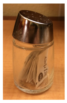
`[ ]` versus `[[ ]]`

x[1] is a pepper shaker containing the first packet of pepper.

`[ ]` versus `[[ ]]`

x[2] is what?

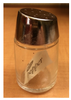
`[ ]` versus `[[ ]]`

x[[1]] is what?

`[ ]` versus `[[ ]]`

x[[1]][[1]] is what?

Data Frames

Let’s relate list()s to our favorite R object: data.frame()s!

data.frame()s are list()s.
Each variable of a data.frame() is an atomic vector().
The vector()s all have the same length but not necessary the same class.

Data Frames

my_pets

    name type age birthplace
1   Dude  dog   8 Washington
2 Pickle  cat   6       <NA>
3   Kyle  cat   4       Utah
4   Nubs  cat  NA       <NA>

my_pets$name

[1] "Dude"   "Pickle" "Kyle"   "Nubs"

Data Frames

str(my_pets[1])

'data.frame':   4 obs. of  1 variable:
 $ name: chr  "Dude" "Pickle" "Kyle" "Nubs"

str(my_pets[[1]])

 chr [1:4] "Dude" "Pickle" "Kyle" "Nubs"

my_pets[1, 2]

[1] "dog"

my_pets[1, ]

  name type age birthplace
1 Dude  dog   8 Washington

Thoughts about R data objects

We can create and interact with (atomic) vectors and lists (generic vectors).
When writing and debugging code, it is a good idea to check the class() of an object.
R will sometimes change the type of an object without telling us (but based on our actions).
Vectorization makes R code speedy but also can cause you to do something you didn’t mean to do.
While we will primarily interact with vector()s and data.frame()s, we will sometimes need list()s.

Next time

Joining, reshaping, and tidying data!

Next Week

Spatial data in R

Announcements

Week 4 Goals

Looking Ahead to Project 1

What We Need First

dplyr review

Data: Census 2000 (from openintro)

select()

select()

mutate()

filter()

arrange()

arrange()

arrange()

summarize()

group_by() + summarize()

Tip: count()

group_by() + mutate()

group_by() + mutate()

group_by() + mutate()

Now: type of data objects

Math 241 R Data Objects So Far:

R Objects: Vectors

Deep Dive into (atomic) vectors

Flavors of Atomic Vectors

Factors versus Characters

Concatenation

Checking Type

Checking Type

Type Coercion

Operator Coercion

Changing Type

Vectorized

Vectorized: Caution

Recycling

Indexing a Vector

So what about generic vectors/lists?

Lists

Lists

Indexing lists

[ ] versus [[ ]]

[ ] versus [[ ]]

[ ] versus [[ ]]

[ ] versus [[ ]]

[ ] versus [[ ]]

Data Frames

Data Frames

Data Frames

Thoughts about R data objects

Next time

Next Week

`dplyr` review

Data: Census 2000 (from `openintro`)

`select()`

`select()`

`mutate()`

`filter()`

`arrange()`

`arrange()`

`arrange()`

`summarize()`

`group_by()` + `summarize()`

Tip: `count()`

`group_by()` + `mutate()`

`group_by()` + `mutate()`

`group_by()` + `mutate()`

Math 241 `R` Data Objects So Far:

`[ ]` versus `[[ ]]`

`[ ]` versus `[[ ]]`

`[ ]` versus `[[ ]]`

`[ ]` versus `[[ ]]`

`[ ]` versus `[[ ]]`