Joining and Reshaping Data

Grayson White

Math 241
Week 4 | Spring 2026

Announcements

Problem Set 2 is due tomorrow at 9am on Gradescope and Github!

Week 4 Goals

Mon Lecture

Different types of data in R
- atomic and generic vectors
- subsetting objects
Talk more about logical statements
More practice with dplyr verbs and data wrangling

Wed Lecture

Joining multiple data frames
“Tidy” data
Reshaping data frames

First: Coding Style

“Good coding style is like correct punctuation: you can manage without it, butitsuremakesthingseasiertoread.” – The Tidyverse Style Guide

messy4324 <-select(dataset,thing1,thing2)%>%filter(thing1=="uncool")

clean <- select(dataset, thing1, thing2) %>%
  filter(thing1 == "uncool")

Coding Style

Part of writing easily reproducible code.
Lots of reasonable coding styles.
Important piece is consistency across all coders on a project.
Some suggestions:
- Use spaces liberally.
- Let R help you with the proper indenting.
- Think carefully about names.
Check out the Tidyverse Style Guide.

A cautionary tale: `tibble`()s vs. `data.frame`()s

Tibbles are a special type of data frame that come with the tidyverse
They have nicer printing behavior, and, as mentioned briefly last class, a different subsetting behavior.
Let’s look at an example:

library(tidyverse)
boop <- data.frame(x = 1:3, y = c("cat", "dog", "bird"))
beep <- tibble(x = 1:3, y = c("cat", "dog", "bird"))

boop

  x    y
1 1  cat
2 2  dog
3 3 bird

beep

# A tibble: 3 × 2
      x y    
  <int> <chr>
1     1 cat  
2     2 dog  
3     3 bird

A cautionary tale: `tibble`()s vs. `data.frame`()s

boop[2]

     y
1  cat
2  dog
3 bird

class(boop[2])

[1] "data.frame"

beep[2]

# A tibble: 3 × 1
  y    
  <chr>
1 cat  
2 dog  
3 bird

class(beep[2])

[1] "tbl_df"     "tbl"        "data.frame"

boop[1, 2]

[1] "cat"

class(boop[1, 2])

[1] "character"

beep[1, 2]

# A tibble: 1 × 1
  y    
  <chr>
1 cat

class(beep[1, 2])

[1] "tbl_df"     "tbl"        "data.frame"

boop[[1, 2]]

[1] "cat"

beep[[1, 2]]

[1] "cat"

A cautionary tale: `tibble`()s vs. `data.frame`()s

tibble()s have subsetting behavior that is consistent with list()s
And even though data.frame()s are lists, they do not have this consistent behavior
This is frustrating! Be careful.

Relational Data

Most organizations that have a fair amount of data don’t store that data in a single table.
- Think Google, Facebook, LinkedIn, …
Instead, they use a relational database: collection of linkable tables that are linked together by keys.

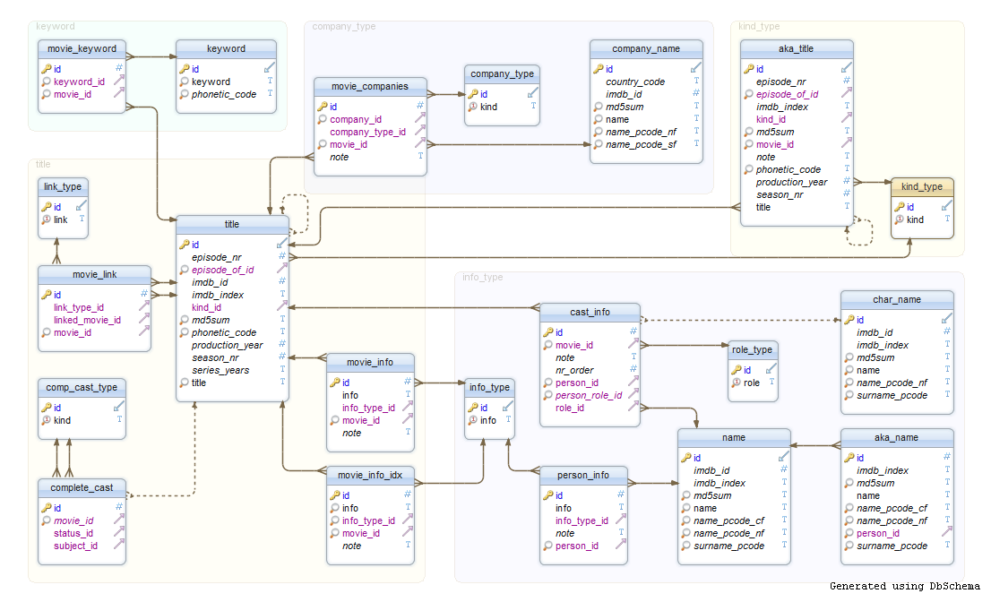
Typically use a SQL server for storing and managing that data.
We are going to learn to how to join relational data in R using dplyr.
- Towards the end of the semester, we’ll learn some SQL. It is very similar to dplyr.

Data Joins in `R`

Today, we’ll look at a few ways to join the following tables x and y:

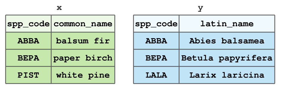
Small dataset of tree types for illustrative purposes.
In Problem Set 3, you’ll get good experience joining larger datasets.

Motivating example: forest inventory

It is common in forestry, and in particular forest inventory, to have multiple data frames where data are stored due to a variety of factors.
In order to perform most statistical analyses, you must have the necessary data in one data frame.
Example: the US Forest Service, Forest Inventory & Analysis stores plot-level, tree-level, subplot-level, … data in one database. Researchers must combine these data into a singular table to do analyses.

Types of Data Joins

The dplyr package, which is part of the tidyverse, includes functions for two general types of joins:

Mutating joins, which combine the columns of data frames x and y, and
Filtering joins, which match the rows of data frames x and y.

Think of how mutate() adds columns to a data frame, while filter() removes rows.

Example Data

For the following examples of data joins, we will use the data frames from the first slide. We can load this data into R:

library(tidyverse)
x <- data.frame(spp_code = c("ABBA", "BEPA", "PIST"),
                common_name = c("balsum fir", "paper birch", "white pine"))

y <- data.frame(spp_code = c("ABBA", "BEPA", "LALA"),
                latin_name = c("Abies balsamea", 
                               "Betula papyrifera",
                               "Larix laricina"))

Mutating Joins

dplyr contains four mutating joins:

left_join(x, y) keeps all rows of x, but if a row in y does not match to x, an NA is assigned to that row in the new columns.
right_join(x, y) is equivalent to left_join(y, x), except for column order.
inner_join(x, y) keeps only the rows matched between x and y.
full_join(x, y) keeps all rows of both x and y.

Examples: Mutating Joins

Recall our example data

  spp_code common_name
1     ABBA  balsum fir
2     BEPA paper birch
3     PIST  white pine

  spp_code        latin_name
1     ABBA    Abies balsamea
2     BEPA Betula papyrifera
3     LALA    Larix laricina

`left_join()`

left_join(x, y)

Joining with `by = join_by(spp_code)`

  spp_code common_name        latin_name
1     ABBA  balsum fir    Abies balsamea
2     BEPA paper birch Betula papyrifera
3     PIST  white pine              <NA>

`left_join()`

left_join(x, y)

Joining with `by = join_by(spp_code)`

  spp_code common_name        latin_name
1     ABBA  balsum fir    Abies balsamea
2     BEPA paper birch Betula papyrifera
3     PIST  white pine              <NA>

But what’s that message about?

"Joining with `by = join_by(spp_code)`"

We need to specify a key 🔑

A key is can just be thought of the name(s) of the column(s) you’re joining by. In the left_join() from the last slide, R assumed we were joining by the column spp_code since both x and y have a column with that name.

Keys are important, especially when the columns you are joining by have different names, or you are joining by multiple columns.

`left_join()`, with a 🔑

left_join(x, y, by = "spp_code")

  spp_code common_name        latin_name
1     ABBA  balsum fir    Abies balsamea
2     BEPA paper birch Betula papyrifera
3     PIST  white pine              <NA>

Notice that we specify this key with the by argument. This is the same for all joins in dplyr.

`right_join()`

right_join(y, x, by = "spp_code")

  spp_code        latin_name common_name
1     ABBA    Abies balsamea  balsum fir
2     BEPA Betula papyrifera paper birch
3     PIST              <NA>  white pine

`right_join()`

right_join(y, x, by = "spp_code")

  spp_code        latin_name common_name
1     ABBA    Abies balsamea  balsum fir
2     BEPA Betula papyrifera paper birch
3     PIST              <NA>  white pine

Notice that this is the same as our previous left_join().

What happens if we try switching the order of x and y?

right_join(x, y, by = "spp_code")

`right_join()`

right_join(y, x, by = "spp_code")

  spp_code        latin_name common_name
1     ABBA    Abies balsamea  balsum fir
2     BEPA Betula papyrifera paper birch
3     PIST              <NA>  white pine

Notice that this is the same as our previous left_join().

What happens if we try switching the order of x and y?

right_join(x, y, by = "spp_code")

  spp_code common_name        latin_name
1     ABBA  balsum fir    Abies balsamea
2     BEPA paper birch Betula papyrifera
3     LALA        <NA>    Larix laricina

`inner_join()`

How many rows will the output have?

inner_join(x, y, by = "spp_code")

`inner_join()`

How many rows will the output have?

inner_join(x, y, by = "spp_code")

  spp_code common_name        latin_name
1     ABBA  balsum fir    Abies balsamea
2     BEPA paper birch Betula papyrifera

Why is this the result?

`full_join()`

How many rows will the output have?

full_join(x, y, by = "spp_code")

`full_join()`

How many rows will the output have?

full_join(x, y, by = "spp_code")

  spp_code common_name        latin_name
1     ABBA  balsum fir    Abies balsamea
2     BEPA paper birch Betula papyrifera
3     PIST  white pine              <NA>
4     LALA        <NA>    Larix laricina

Why is this the result?

Filtering Joins

dplyr contains two filtering joins:

semi_join(x, y) keeps all the rows in x that have a match in y.
anti_join(x, y) removes all the rows in x that have a match in y.

Note: Unlike mutating joins, filtering joins do not add any columns to the data.

`semi_join()`

How many rows will this semi_join return? How many columns?

semi_join(x, y, by = "spp_code")

`semi_join()`

How many rows will this semi_join return? How many columns?

semi_join(x, y, by = "spp_code")

  spp_code common_name
1     ABBA  balsum fir
2     BEPA paper birch

`semi_join()`

What about this semi_join? Will it be the same as semi_join(x, y)?

semi_join(y, x, by = "spp_code")

`semi_join()`

What about this semi_join? Will it be the same as semi_join(x, y)?

semi_join(y, x, by = "spp_code")

  spp_code        latin_name
1     ABBA    Abies balsamea
2     BEPA Betula papyrifera

`anti_join()`

Let’s see what anti_join does:

anti_join(x, y, by = "spp_code")

`anti_join()`

Let’s see what anti_join does:

anti_join(x, y, by = "spp_code")

  spp_code common_name
1     PIST  white pine

Why do we get this output?

`anti_join()`

What happens if we switch the order of x and y?

anti_join(y, x, by = "spp_code")

`anti_join()`

What happens if we switch the order of x and y?

anti_join(y, x, by = "spp_code")

  spp_code     latin_name
1     LALA Larix laricina

An Important Subtlety: Column Names

So far, we have joined x and y by the spp_code column.

But what if y had the same column named differently:

y <- y %>%
  rename(species_code = spp_code)
y

  species_code        latin_name
1         ABBA    Abies balsamea
2         BEPA Betula papyrifera
3         LALA    Larix laricina

How Do We Join `x` and `y`?

left_join(x, y)

Error in `left_join()`:
! `by` must be supplied when `x` and `y` have no common variables.
ℹ Use `cross_join()` to perform a cross-join.

Looks like we need to specify by (our 🔑)

How Do We Join `x` and `y`?

left_join(x, y)

Error in `left_join()`:
! `by` must be supplied when `x` and `y` have no common variables.
ℹ Use `cross_join()` to perform a cross-join.

Looks like we need to specify by (our 🔑)

left_join(x, y, by = "spp_code")

Error in `left_join()`:
! Join columns in `y` must be present in the data.
✖ Problem with `spp_code`.

Still not working!

How Do We Join `x` and `y`?

left_join(x, y)

Error in `left_join()`:
! `by` must be supplied when `x` and `y` have no common variables.
ℹ Use `cross_join()` to perform a cross-join.

Looks like we need to specify by (our 🔑)

left_join(x, y, by = "spp_code")

Error in `left_join()`:
! Join columns in `y` must be present in the data.
✖ Problem with `spp_code`.

Still not working!

left_join(x, y, by = c("spp_code" = "species_code"))

  spp_code common_name        latin_name
1     ABBA  balsum fir    Abies balsamea
2     BEPA paper birch Betula papyrifera
3     PIST  white pine              <NA>

Now: reshaping data

Data Wrangling in the `tidyverse`

Question: Why do we need TWO different data wrangling packages in the tidyverse?

Question: What does dplyr do?

Performs various data manipulation tasks, such as extracting and summarizing

Question: So what is left for tidyr to do?

Reshape data into different formats (e.g. long and wide)

Key Idea: Reshape Data to a Tidy Data Format

“Happy families are all alike; every unhappy family is unhappy in its own way.” – Leo Tolstoy

“Tidy datasets are all alike, but every messy dataset is messy in its own way.” – Hadley Wickham

By tidy, we don’t mean neat.
Tidy data satisfy rules that make it easy to work with the data.

Tidy Data Rules

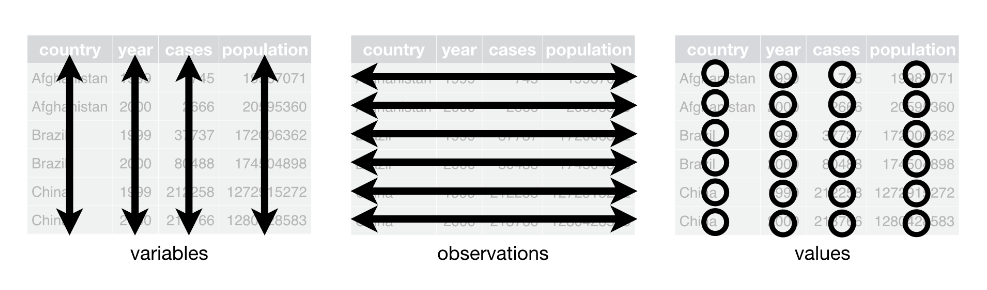
Each column is a single variable.
Each row is a unique observation.
Each value must have its own cell.
See this blog post for a cute introduction to “tidy data”.

Tidy Data

  spp_code common_name
1     ABBA  balsum fir
2     BEPA paper birch
3     PIST  white pine

Un-Tidy Data

The face dataset from IFDAR:

face <- read_csv("data/FACE_aspen_core_growth.csv") %>%
  select(Rep, Treat, Clone, ID = `ID #`,
        contains(as.character(2001:2005)) & contains("Height"))
glimpse(face)

Rows: 1,991
Columns: 9
$ Rep           <dbl> 1, 1, 1, 1, 1, 1, 1, 1, 1, 1, 1, 1, 1, 1, 1, 1, 1, 1, 1,…
$ Treat         <dbl> 1, 1, 1, 1, 1, 1, 1, 1, 1, 1, 1, 1, 1, 1, 1, 1, 1, 1, 1,…
$ Clone         <dbl> 8, 216, 8, 216, 216, 271, 271, 8, 259, 271, 271, 271, 27…
$ ID            <dbl> 45, 44, 43, 42, 54, 55, 56, 57, 58, 59, 60, 73, 72, 71, …
$ `2001_Height` <dbl> NA, 547, 273, 526, 328, 543, 450, 217, 158, 230, NA, 516…
$ `2002_Height` <dbl> NA, 622, 275, 619, 341, 590, 502, 227, 155, 241, NA, 619…
$ `2003_Height` <dbl> NA, 715, 305, 720, 364, 634, 587, 256, NA, 260, NA, 742,…
$ `2004_Height` <dbl> NA, 716, 324, 706, 361, 691, 639, 266, NA, 263, NA, 703,…
$ `2005_Height` <dbl> NA, 817, 323, 738, 366, 669, 647, 269, NA, 270, NA, 862,…

Data on tree diameter measurements in a study assessing the effects of different gasses on tree growth.

FACE data

face

# A tibble: 1,991 × 9
     Rep Treat Clone    ID `2001_Height` `2002_Height` `2003_Height`
   <dbl> <dbl> <dbl> <dbl>         <dbl>         <dbl>         <dbl>
 1     1     1     8    45            NA            NA            NA
 2     1     1   216    44           547           622           715
 3     1     1     8    43           273           275           305
 4     1     1   216    42           526           619           720
 5     1     1   216    54           328           341           364
 6     1     1   271    55           543           590           634
 7     1     1   271    56           450           502           587
 8     1     1     8    57           217           227           256
 9     1     1   259    58           158           155            NA
10     1     1   271    59           230           241           260
# ℹ 1,981 more rows
# ℹ 2 more variables: `2004_Height` <dbl>, `2005_Height` <dbl>

What does a row represent?
What does a column represent?

How do we make this data tidy? 🤔

face

# A tibble: 1,991 × 9
     Rep Treat Clone    ID `2001_Height` `2002_Height` `2003_Height`
   <dbl> <dbl> <dbl> <dbl>         <dbl>         <dbl>         <dbl>
 1     1     1     8    45            NA            NA            NA
 2     1     1   216    44           547           622           715
 3     1     1     8    43           273           275           305
 4     1     1   216    42           526           619           720
 5     1     1   216    54           328           341           364
 6     1     1   271    55           543           590           634
 7     1     1   271    56           450           502           587
 8     1     1     8    57           217           227           256
 9     1     1   259    58           158           155            NA
10     1     1   271    59           230           241           260
# ℹ 1,981 more rows
# ℹ 2 more variables: `2004_Height` <dbl>, `2005_Height` <dbl>

Each row should represent a measurement for a given rep, treatment, clone, and ID. But currently, we have multiple measurements on the same row.
Further, we have multiple columns for the “height” variable.
Not tidy!

We need to pivot the data into a longer format!

Enter, pivot_longer().

pivot_longer(), a function from tidyr takes four key arguments:

.data: the data you’d like to pivot,
cols: the columns you’d like to pivot,
names_to: the new column that will be created which takes the column names from cols as values, and
values_to: the new column that will be created which takes the column values from cols as values.

Why the long `face`?

face_long <- face %>%
  pivot_longer(
    cols = c("2001_Height", "2002_Height", "2003_Height", 
             "2004_Height", "2005_Height"),
    names_to = "Year_Type",
    values_to = "Height_cm")

Why the long `face`?

face_long <- face %>%
  pivot_longer(
    cols = c("2001_Height", "2002_Height", "2003_Height", 
             "2004_Height", "2005_Height"),
    names_to = "Year_Type",
    values_to = "Height_cm")

Why the long `face`?

face_long <- face %>%
  pivot_longer(
    cols = contains("Height"),
    names_to = "Year_Type",
    values_to = "Height_cm")

A cleaner way to select these columns is to use dplyr’s contains() function.

Why the long `face`?

face_long

# A tibble: 9,955 × 6
     Rep Treat Clone    ID Year_Type   Height_cm
   <dbl> <dbl> <dbl> <dbl> <chr>           <dbl>
 1     1     1     8    45 2001_Height        NA
 2     1     1     8    45 2002_Height        NA
 3     1     1     8    45 2003_Height        NA
 4     1     1     8    45 2004_Height        NA
 5     1     1     8    45 2005_Height        NA
 6     1     1   216    44 2001_Height       547
 7     1     1   216    44 2002_Height       622
 8     1     1   216    44 2003_Height       715
 9     1     1   216    44 2004_Height       716
10     1     1   216    44 2005_Height       817
# ℹ 9,945 more rows

To get tidy data!

Going (back) to wide data

Sometimes, we need to “widen” a dataset to get it into tidy format.
For this example, we will just widen the face_long dataset back to its original form.
tidyr has an aptly named function, pivot_wider().
Key arguments of pivot_wider():
- .data: the data frame to widen,
- names_from: the column that contains values which will be assigned as the new column names,
- values_from: the column that contains

Pivoting wider

face_wide <- face_long %>%
  pivot_wider(names_from = "Year_Type", values_from = "Height_cm")

all_equal(face, face_wide)

[1] TRUE

This results in the same data frame that we started with!

Other useful `tidyr` functions

Sometimes, a column represents multiple variables (or only part of a variable!).
So, tidyr has some functions for dealing with that, too:
unite() for pasteing column values together with specified separators,
The separate_wider_*() family: for splitting columns into multiple new columns:
- separate_wider_delim(): separate by delimiter
- separate_wider_position(): separate by position
- separate_wider_regex(): separate by regular expression

`unite()`: examples

face_long

# A tibble: 9,955 × 6
     Rep Treat Clone    ID Year_Type   Height_cm
   <dbl> <dbl> <dbl> <dbl> <chr>           <dbl>
 1     1     1     8    45 2001_Height        NA
 2     1     1     8    45 2002_Height        NA
 3     1     1     8    45 2003_Height        NA
 4     1     1     8    45 2004_Height        NA
 5     1     1     8    45 2005_Height        NA
 6     1     1   216    44 2001_Height       547
 7     1     1   216    44 2002_Height       622
 8     1     1   216    44 2003_Height       715
 9     1     1   216    44 2004_Height       716
10     1     1   216    44 2005_Height       817
# ℹ 9,945 more rows

`unite()`: examples

face_long %>%
  unite(col = "Design", Rep, Treat, Clone, sep = "_")

# A tibble: 9,955 × 4
   Design     ID Year_Type   Height_cm
   <chr>   <dbl> <chr>           <dbl>
 1 1_1_8      45 2001_Height        NA
 2 1_1_8      45 2002_Height        NA
 3 1_1_8      45 2003_Height        NA
 4 1_1_8      45 2004_Height        NA
 5 1_1_8      45 2005_Height        NA
 6 1_1_216    44 2001_Height       547
 7 1_1_216    44 2002_Height       622
 8 1_1_216    44 2003_Height       715
 9 1_1_216    44 2004_Height       716
10 1_1_216    44 2005_Height       817
# ℹ 9,945 more rows

`unite()`: examples

face_long_dot <- face_long %>%
  unite(col = "Design", Rep, Treat, Clone, sep = ".")
face_long_dot

# A tibble: 9,955 × 4
   Design     ID Year_Type   Height_cm
   <chr>   <dbl> <chr>           <dbl>
 1 1.1.8      45 2001_Height        NA
 2 1.1.8      45 2002_Height        NA
 3 1.1.8      45 2003_Height        NA
 4 1.1.8      45 2004_Height        NA
 5 1.1.8      45 2005_Height        NA
 6 1.1.216    44 2001_Height       547
 7 1.1.216    44 2002_Height       622
 8 1.1.216    44 2003_Height       715
 9 1.1.216    44 2004_Height       716
10 1.1.216    44 2005_Height       817
# ℹ 9,945 more rows

`separate_wider_delim()` example

face_long_dot %>%
  separate_wider_delim(cols = "Design", 
                       delim = ".",
                       names = c("Rep", "Treat", "Clone"))

# A tibble: 9,955 × 6
   Rep   Treat Clone    ID Year_Type   Height_cm
   <chr> <chr> <chr> <dbl> <chr>           <dbl>
 1 1     1     8        45 2001_Height        NA
 2 1     1     8        45 2002_Height        NA
 3 1     1     8        45 2003_Height        NA
 4 1     1     8        45 2004_Height        NA
 5 1     1     8        45 2005_Height        NA
 6 1     1     216      44 2001_Height       547
 7 1     1     216      44 2002_Height       622
 8 1     1     216      44 2003_Height       715
 9 1     1     216      44 2004_Height       716
10 1     1     216      44 2005_Height       817
# ℹ 9,945 more rows

Nice trick: remove unnecessary text

head(face_long)

# A tibble: 6 × 6
    Rep Treat Clone    ID Year_Type   Height_cm
  <dbl> <dbl> <dbl> <dbl> <chr>           <dbl>
1     1     1     8    45 2001_Height        NA
2     1     1     8    45 2002_Height        NA
3     1     1     8    45 2003_Height        NA
4     1     1     8    45 2004_Height        NA
5     1     1     8    45 2005_Height        NA
6     1     1   216    44 2001_Height       547

face_long %>%
  separate_wider_delim(cols = "Year_Type", 
                       delim = "_",
                       names = c("Year", NA))

# A tibble: 9,955 × 6
     Rep Treat Clone    ID Year  Height_cm
   <dbl> <dbl> <dbl> <dbl> <chr>     <dbl>
 1     1     1     8    45 2001         NA
 2     1     1     8    45 2002         NA
 3     1     1     8    45 2003         NA
 4     1     1     8    45 2004         NA
 5     1     1     8    45 2005         NA
 6     1     1   216    44 2001        547
 7     1     1   216    44 2002        622
 8     1     1   216    44 2003        715
 9     1     1   216    44 2004        716
10     1     1   216    44 2005        817
# ℹ 9,945 more rows

Next Week

Spatial data in R

Announcements

Week 4 Goals

First: Coding Style

Coding Style

A cautionary tale: tibble()s vs. data.frame()s

A cautionary tale: tibble()s vs. data.frame()s

A cautionary tale: tibble()s vs. data.frame()s

Relational Data

Data Joins in R

Motivating example: forest inventory

Types of Data Joins

Example Data

Mutating Joins

Examples: Mutating Joins

left_join()

left_join()

We need to specify a key 🔑

left_join(), with a 🔑

right_join()

right_join()

right_join()

inner_join()

inner_join()

full_join()

full_join()

Filtering Joins

semi_join()

semi_join()

semi_join()

semi_join()

anti_join()

anti_join()

anti_join()

anti_join()

An Important Subtlety: Column Names

How Do We Join x and y?

How Do We Join x and y?

How Do We Join x and y?

Now: reshaping data

Data Wrangling in the tidyverse

Key Idea: Reshape Data to a Tidy Data Format

Tidy Data Rules

Tidy Data

Un-Tidy Data

FACE data

How do we make this data tidy? 🤔

We need to pivot the data into a longer format!

Why the long face?

Why the long face?

Why the long face?

Why the long face?

Going (back) to wide data

Pivoting wider

Other useful tidyr functions

unite(): examples

unite(): examples

unite(): examples

separate_wider_delim() example

Nice trick: remove unnecessary text

Next Week

A cautionary tale: `tibble`()s vs. `data.frame`()s

A cautionary tale: `tibble`()s vs. `data.frame`()s

A cautionary tale: `tibble`()s vs. `data.frame`()s

Data Joins in `R`

`left_join()`

`left_join()`

`left_join()`, with a 🔑

`right_join()`

`right_join()`

`right_join()`

`inner_join()`

`inner_join()`

`full_join()`

`full_join()`

`semi_join()`

`semi_join()`

`semi_join()`

`semi_join()`

`anti_join()`

`anti_join()`

`anti_join()`

`anti_join()`

How Do We Join `x` and `y`?

How Do We Join `x` and `y`?

How Do We Join `x` and `y`?

Data Wrangling in the `tidyverse`

Why the long `face`?

Why the long `face`?

Why the long `face`?

Why the long `face`?

Other useful `tidyr` functions

`unite()`: examples

`unite()`: examples

`unite()`: examples

`separate_wider_delim()` example