Spatial Data and Mapping
Grayson White
Math 241
Week 5 | Spring 2026
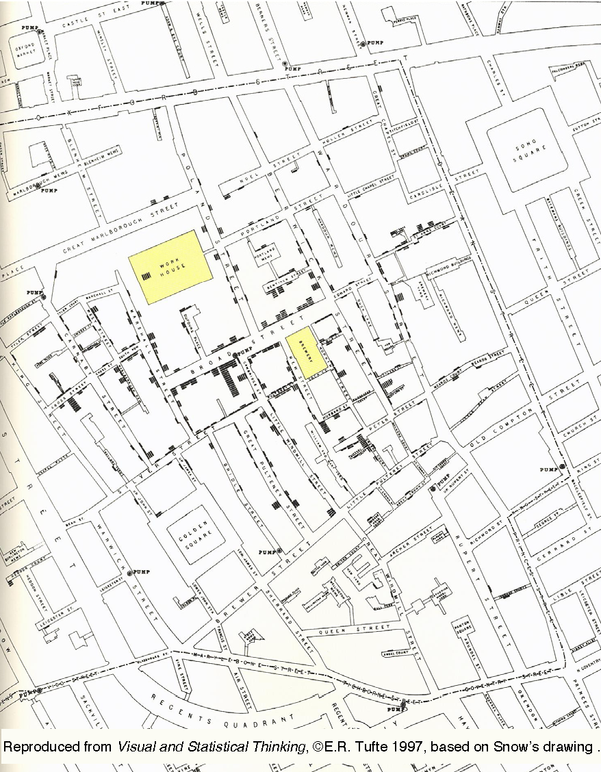
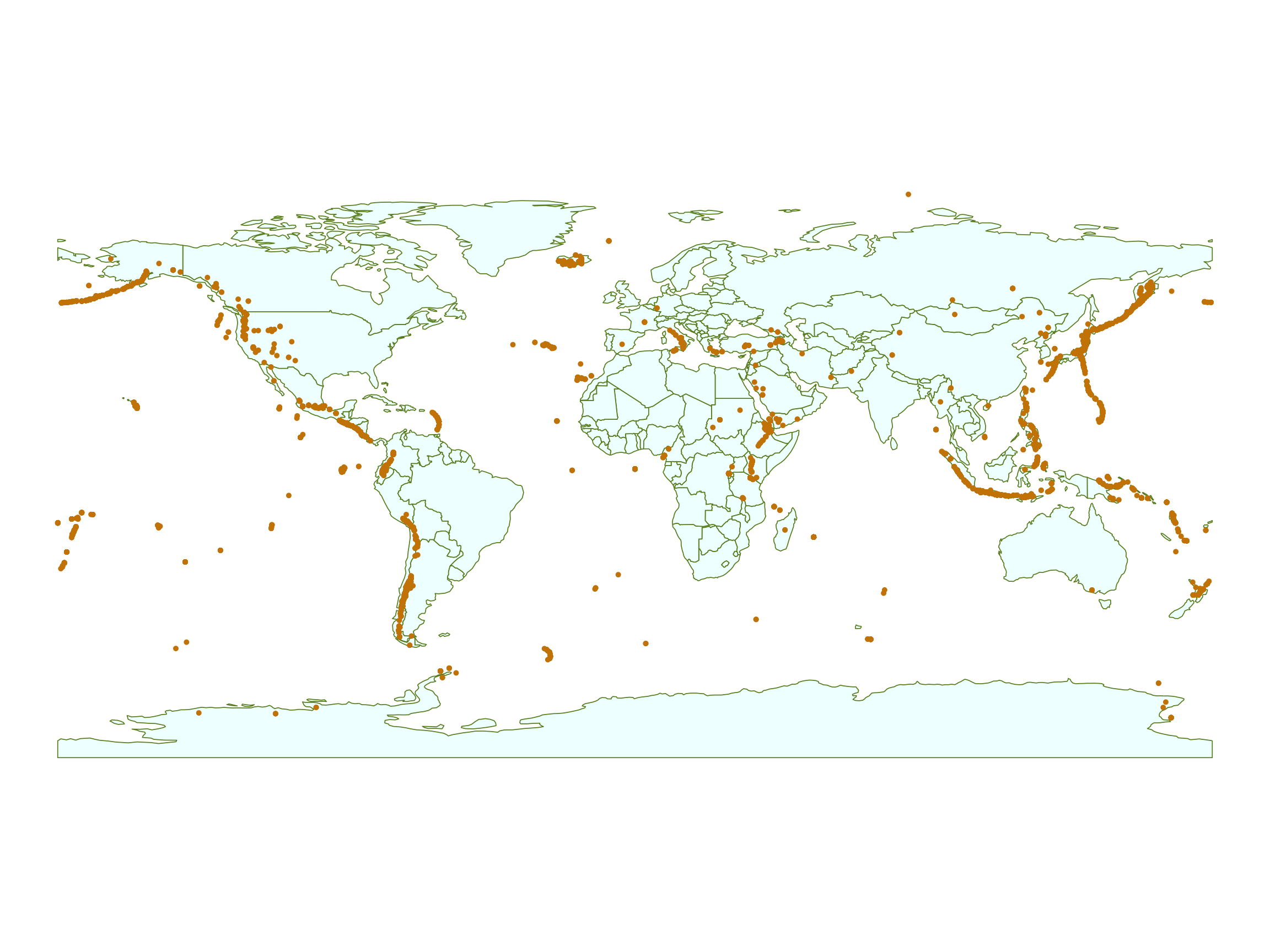
A simple visual model (Tobler 1994):
This figure:
Red Dots: Cholera cases
Blue Triangles: Pumps
Blue Lines: Closest pump is contained in each section
Q: What pattern do you notice?
Q: What are some possible explanations for the “outliers”? (deaths that don’t match up with the pattern)
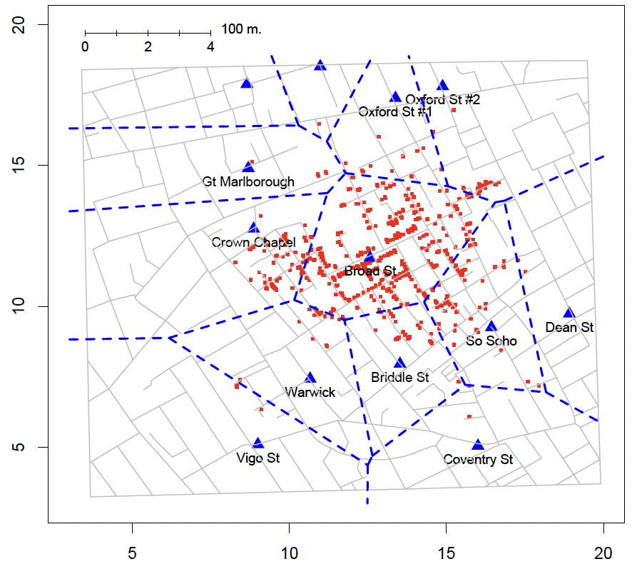
Conclusion: Visualizing spatial data can help us see key patterns
Static Maps
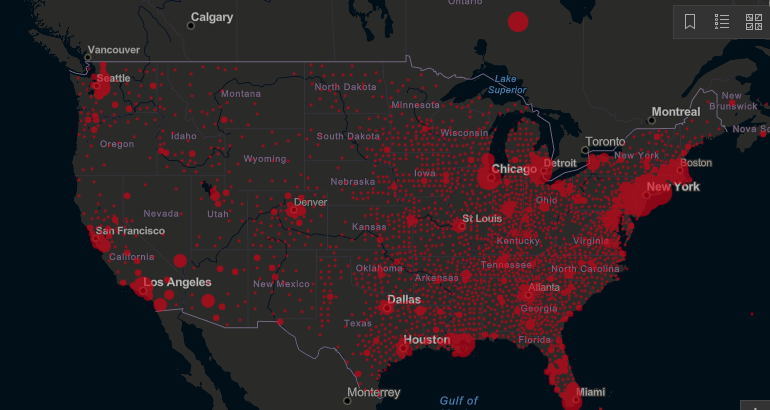
Source: JHU
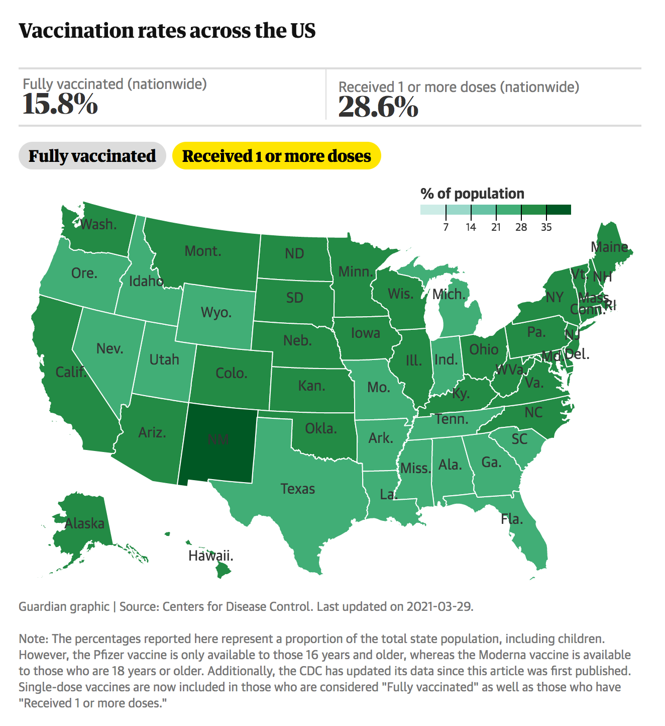
Choropleth Maps
Source: The Guardian
Choropleth Maps
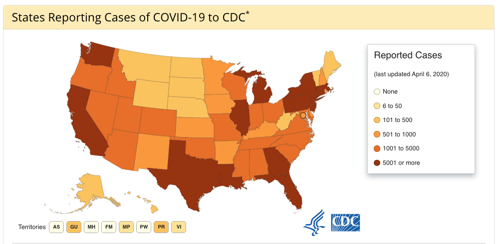
Source: CDC
Choropleth Maps
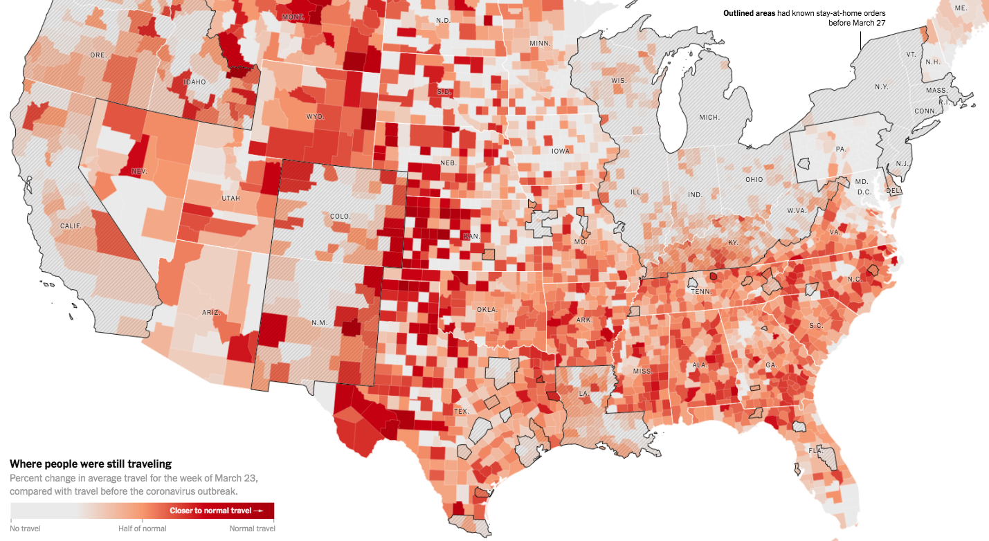
Source: NYtimes.com
Choropleth Maps
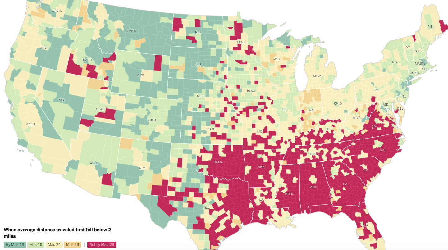
Source: NYtimes.com
Cartogram
Source: Our World in Data
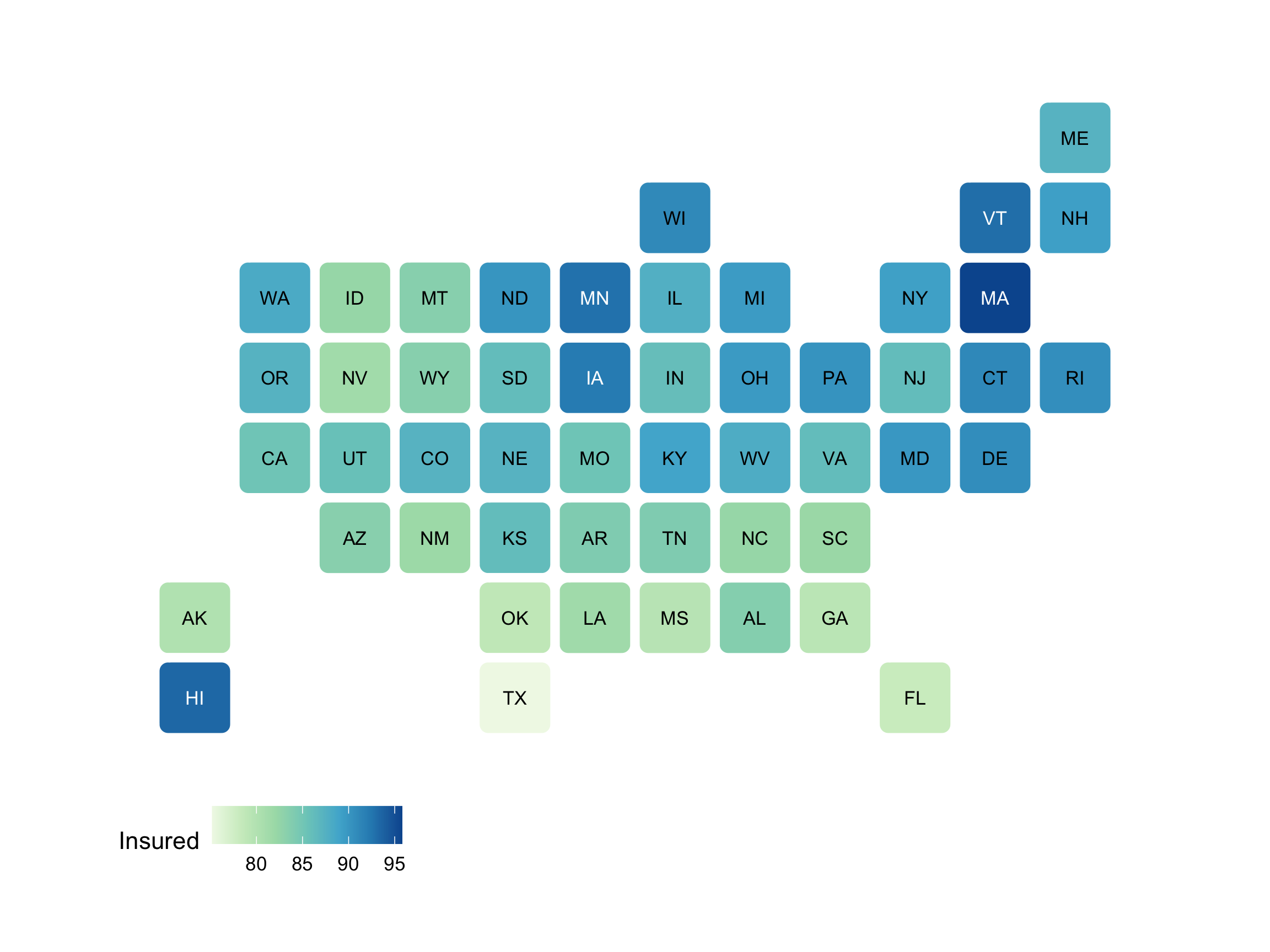
“Hex”bin Maps
Source: FiveThirtyEight
Interactive Maps
Source: NYTimes
What we’ve done so far:
Projections
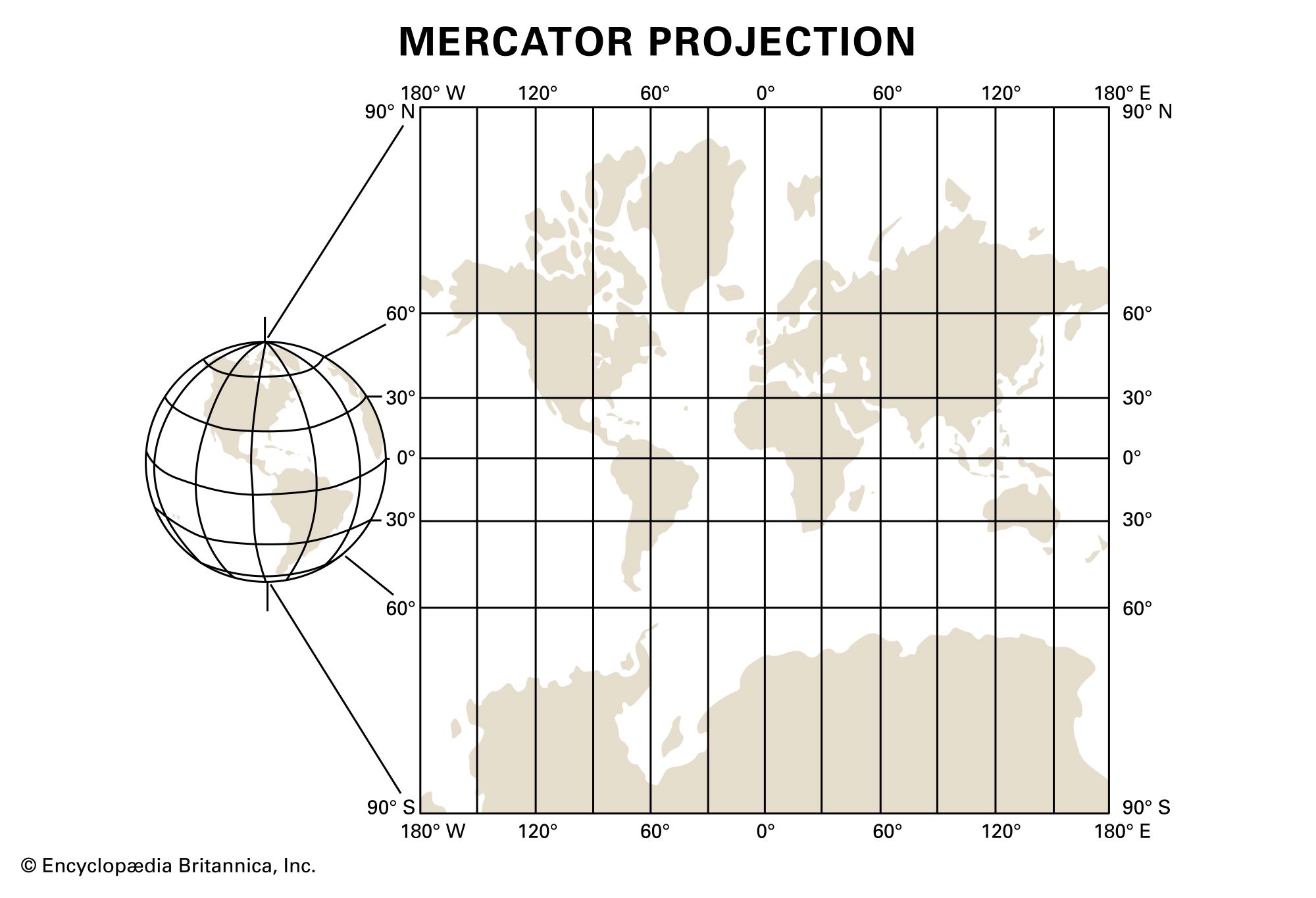
- We live on a globe.
- We like to create maps on flat pages.
- We have to decide how to map things on a globe to a flat page.
- Enter, projections.
Plotting forested_sf


- Preserves relative distances, rather than just plotting on the x/y plane.
Plotting forested_sf
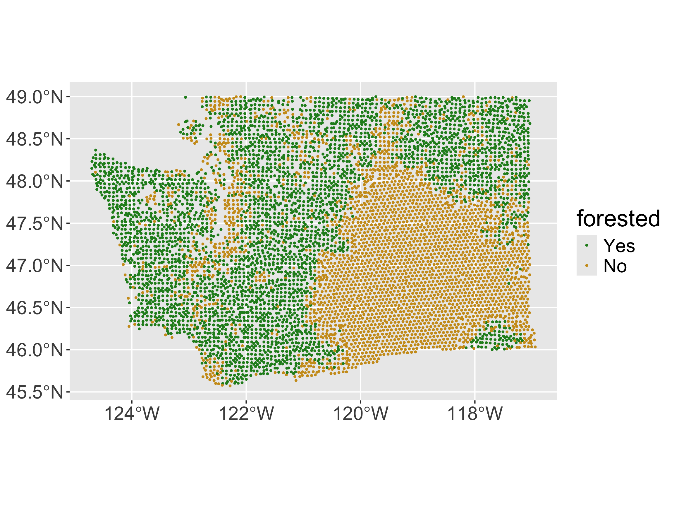
Implicitly,
geom_sf()looks for a geometry column to set its “geometry” aesthetic to.How can we add a base layer?
Polygon Maps
- Want to draw various boundaries
- EXs: Countries, states, counties, etc
- polygon = closed area including the boundaries making up the area
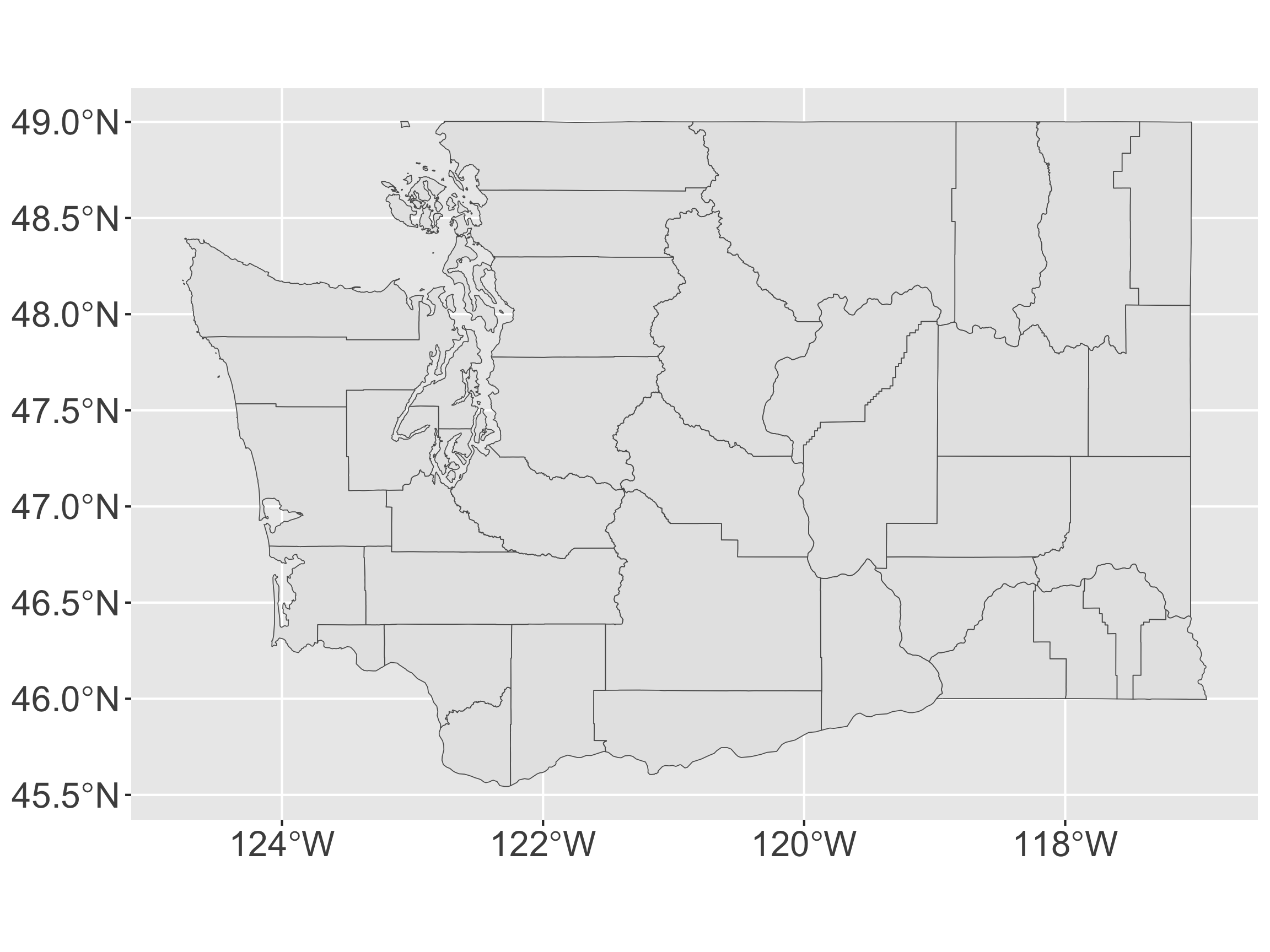
Adding a base layer to our original map
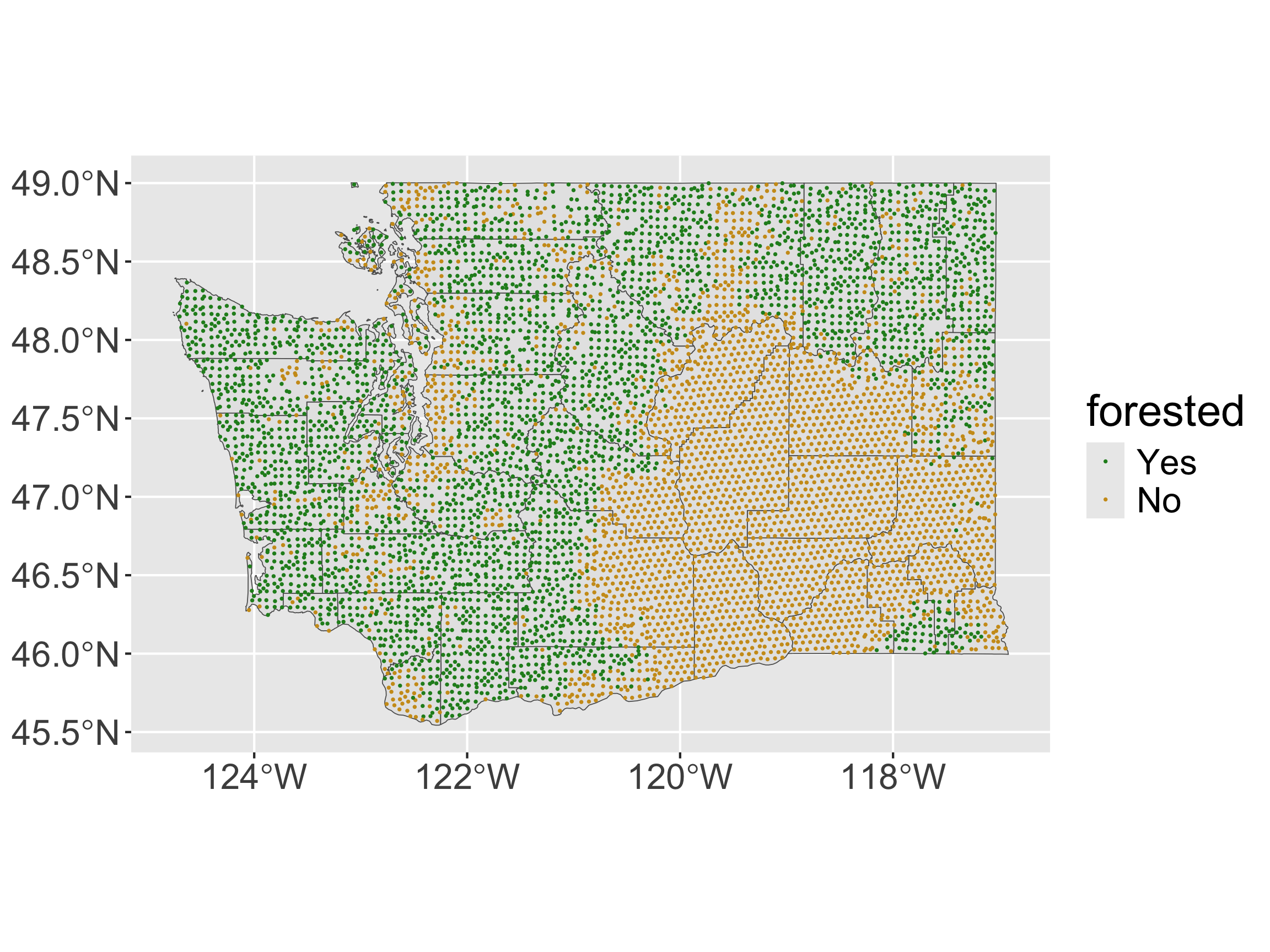
Solution: use the stringr package!
[1] "Thurston" "Island" "Lewis" "Stevens" "Douglas" "San Juan"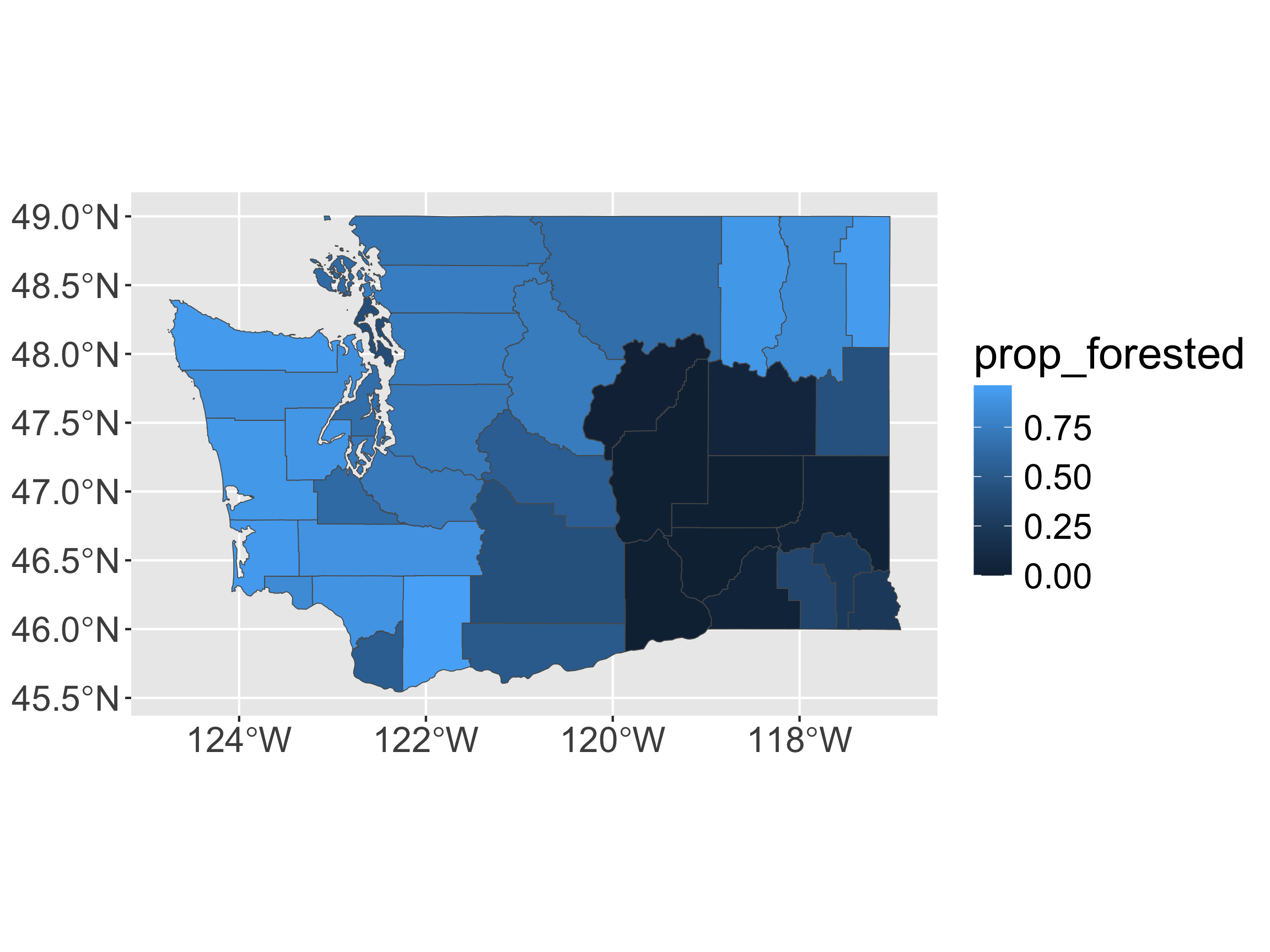
Some mapping suggestions
[1] "Thurston" "Island" "Lewis" "Stevens" "Douglas" "San Juan"# join
left_join(forested_props,
wa,
by = c("county" = "short_name")) %>%
# make R remember this is an sf object
# (R keeps the class of the primary dataset)
st_as_sf() %>%
ggplot(aes(fill = prop_forested)) +
geom_sf() +
scale_fill_distiller(type = "seq",
palette = "Greens",
direction = 1) +
labs(title = "Proportion of forested FIA plots in each county of Washington",
fill = "") +
theme_void() +
theme(legend.position = "right",
legend.key.height = unit(0.9, "in"))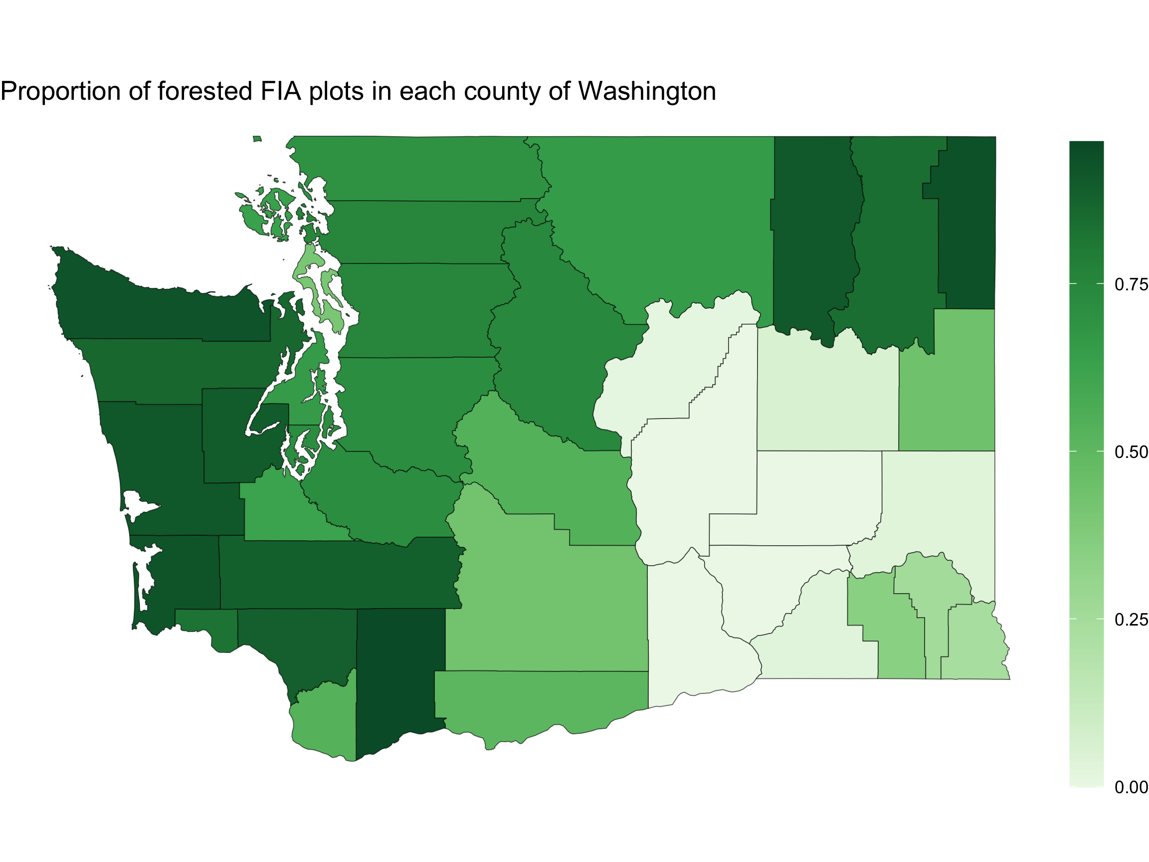
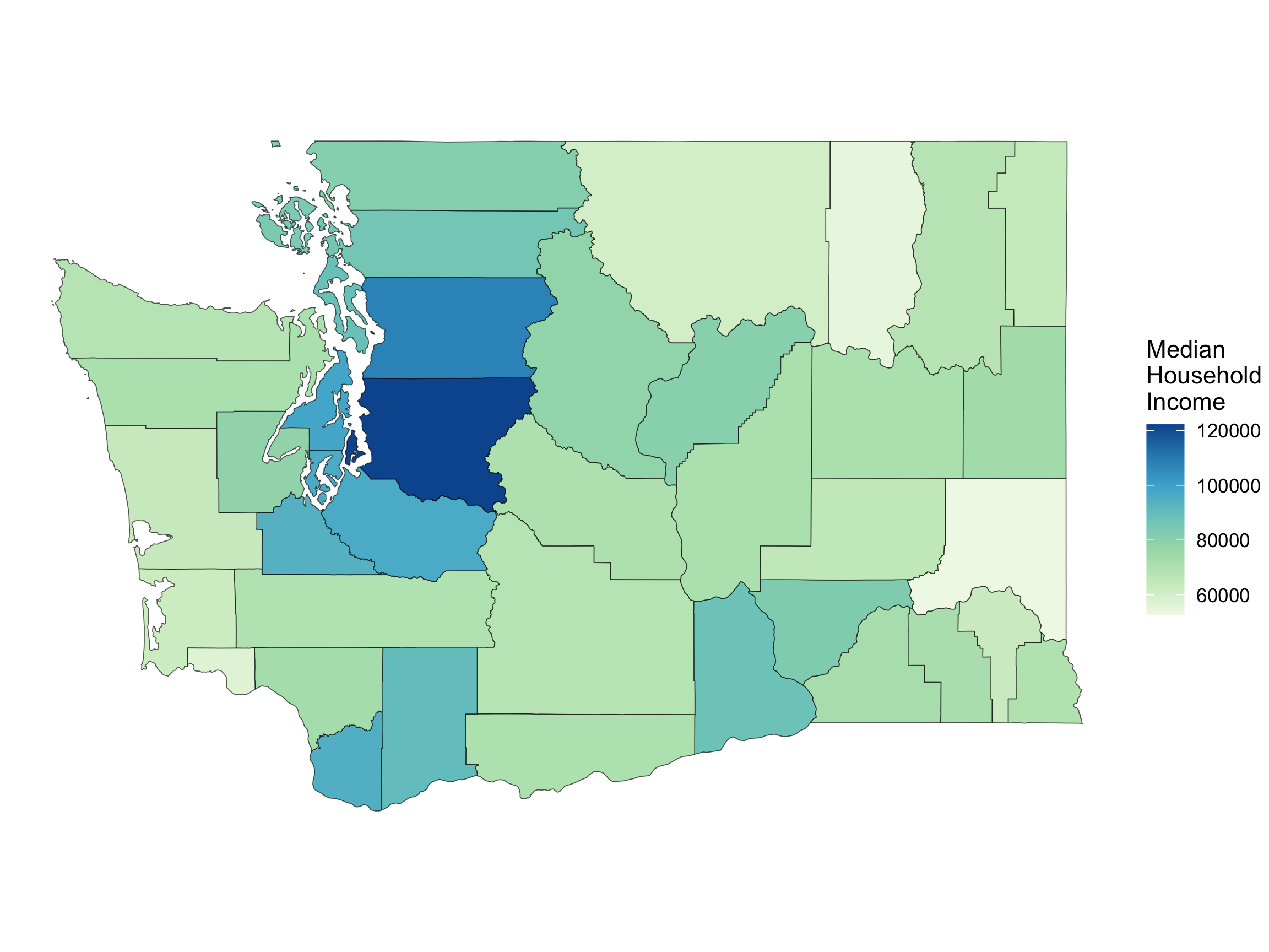
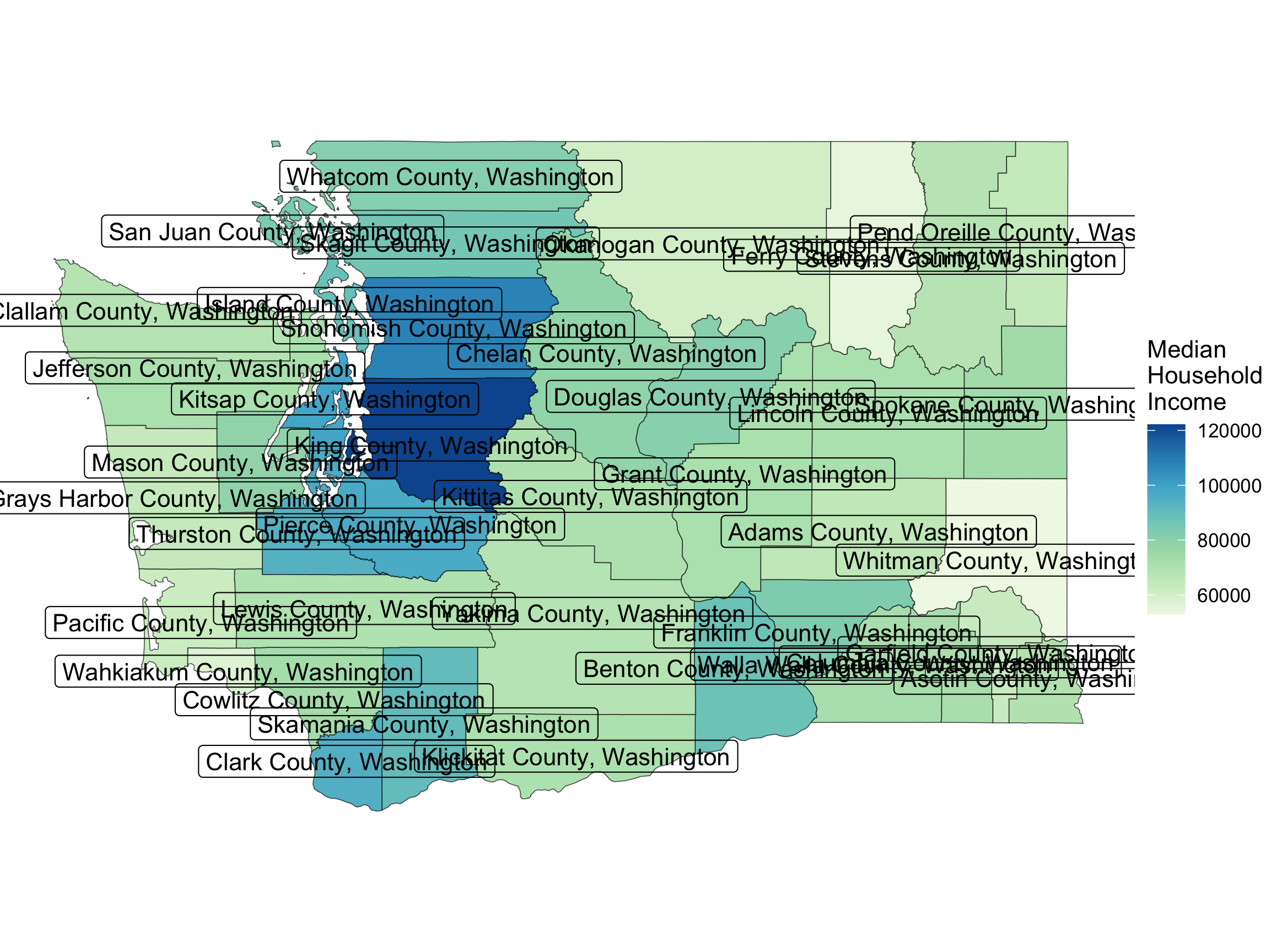
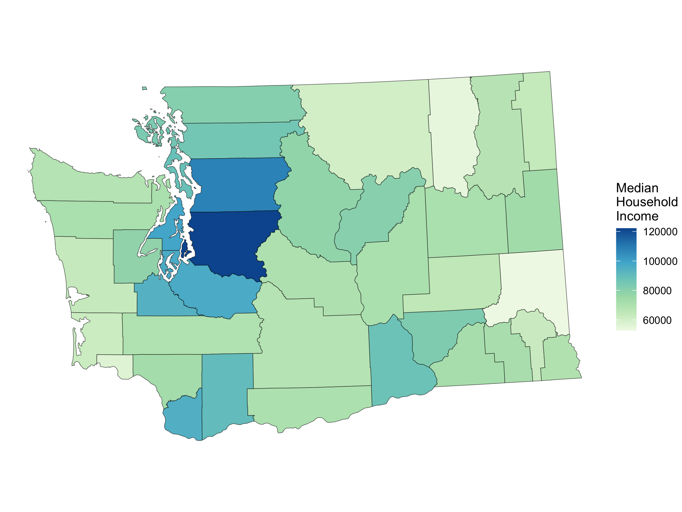
Choropleth Map Showing Median Household Income
Choropleth Map
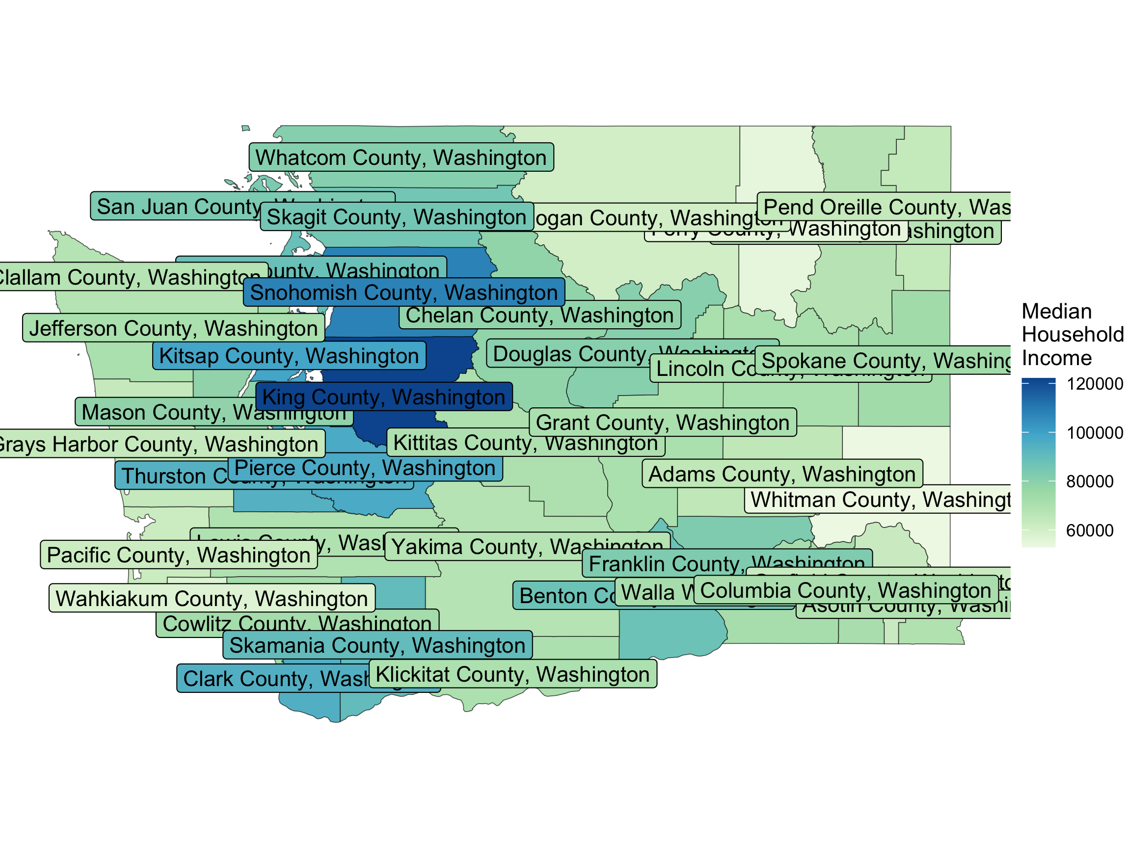
- How should we modify the code if we don’t want the labels to be colored differently?
Choropleth Map
- Fixes for crowding?
Choropleth Map
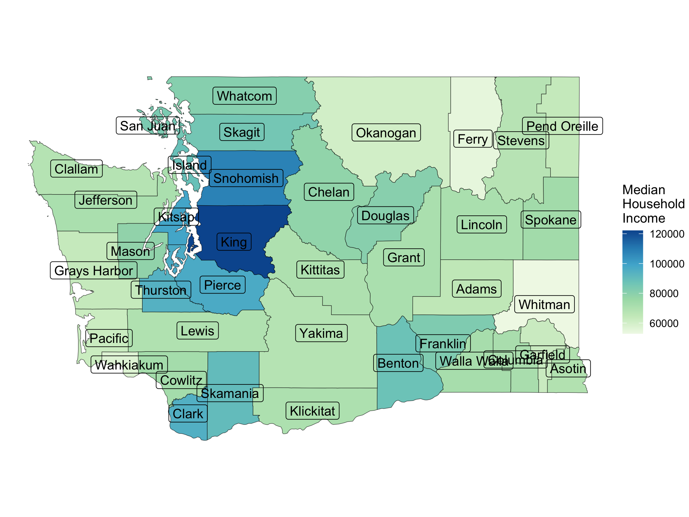
- Fixes for crowding?
Choropleth Map
#devtools::install_github("yutannihilation/ggsflabel")
library(ggsflabel)
ggplot(data = wa,
       mapping =
         aes(geometry = geometry)) +
  geom_sf(mapping =
            aes(fill = estimate)) +
  geom_sf_label_repel(aes(label = short_name),
                      force = 40) +
  scale_fill_distiller(
   name = "Median \nHousehold \nIncome",
   direction = 1, type = "seq", palette = 4) +
  theme_void()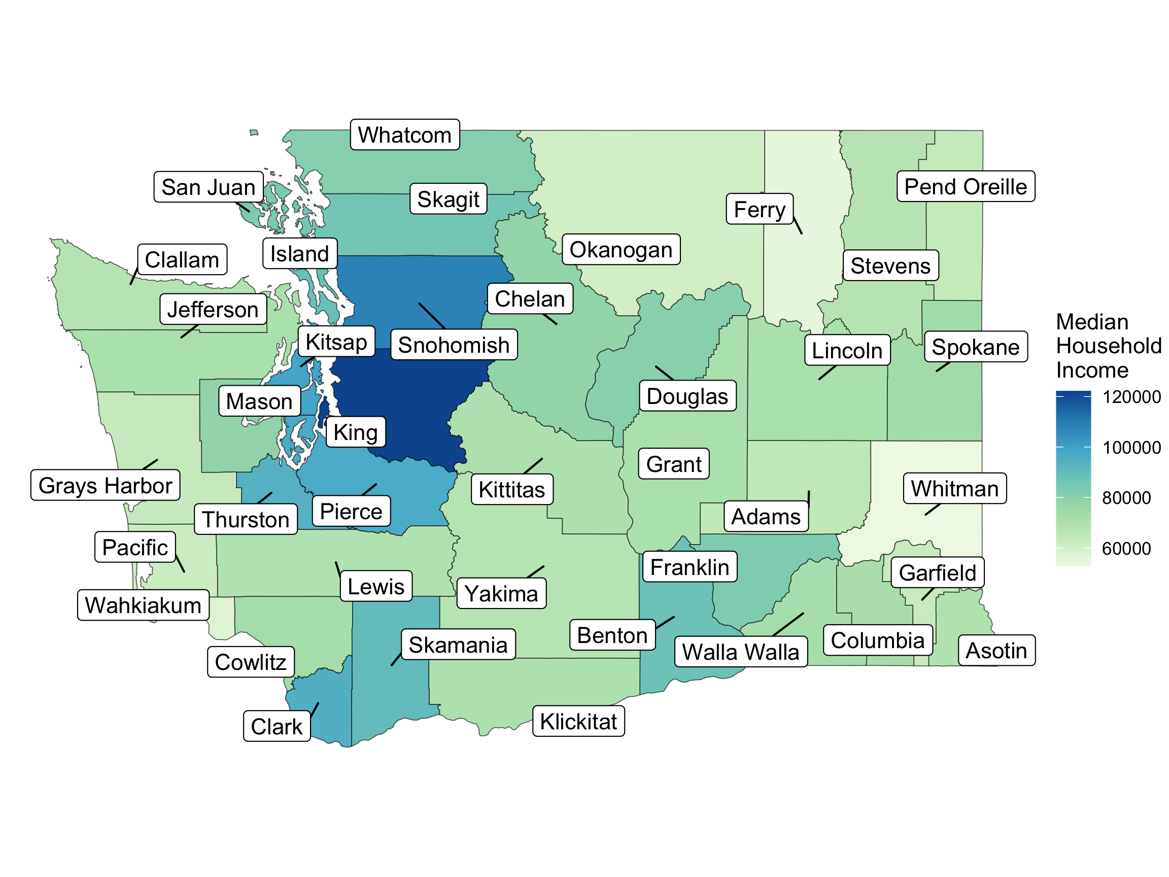
Can Add Information from Another Dataset
library(ggrepel)
ggplot() +
  geom_sf(data = wa,
          mapping =
            aes(geometry = geometry,
                fill = estimate)) +
  geom_point(data = wa_cities,
             mapping = aes(x = long,
                           y = lat),
             shape = 21,
             fill = "white",
             color = "black") +
  geom_label_repel(data = wa_cities,
                   mapping =
                     aes(x = long,
                         y = lat,
                         label = city)) +
  scale_fill_distiller(
   name = "Median \nHousehold \nIncome",
   direction = 1, type = "seq", palette = 4) +
  theme_void()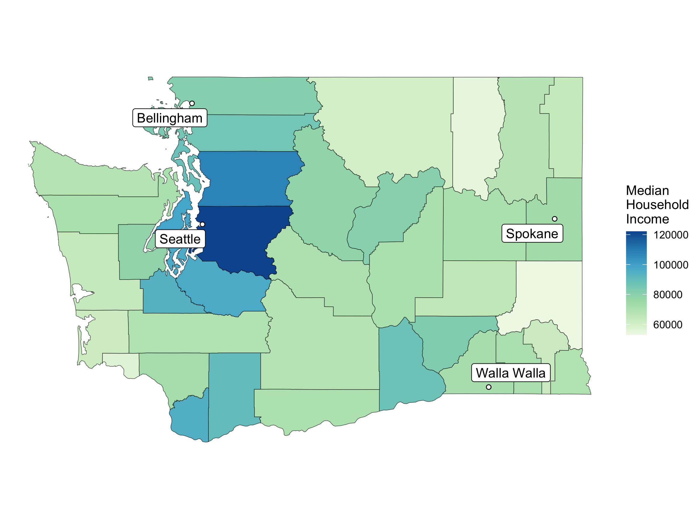
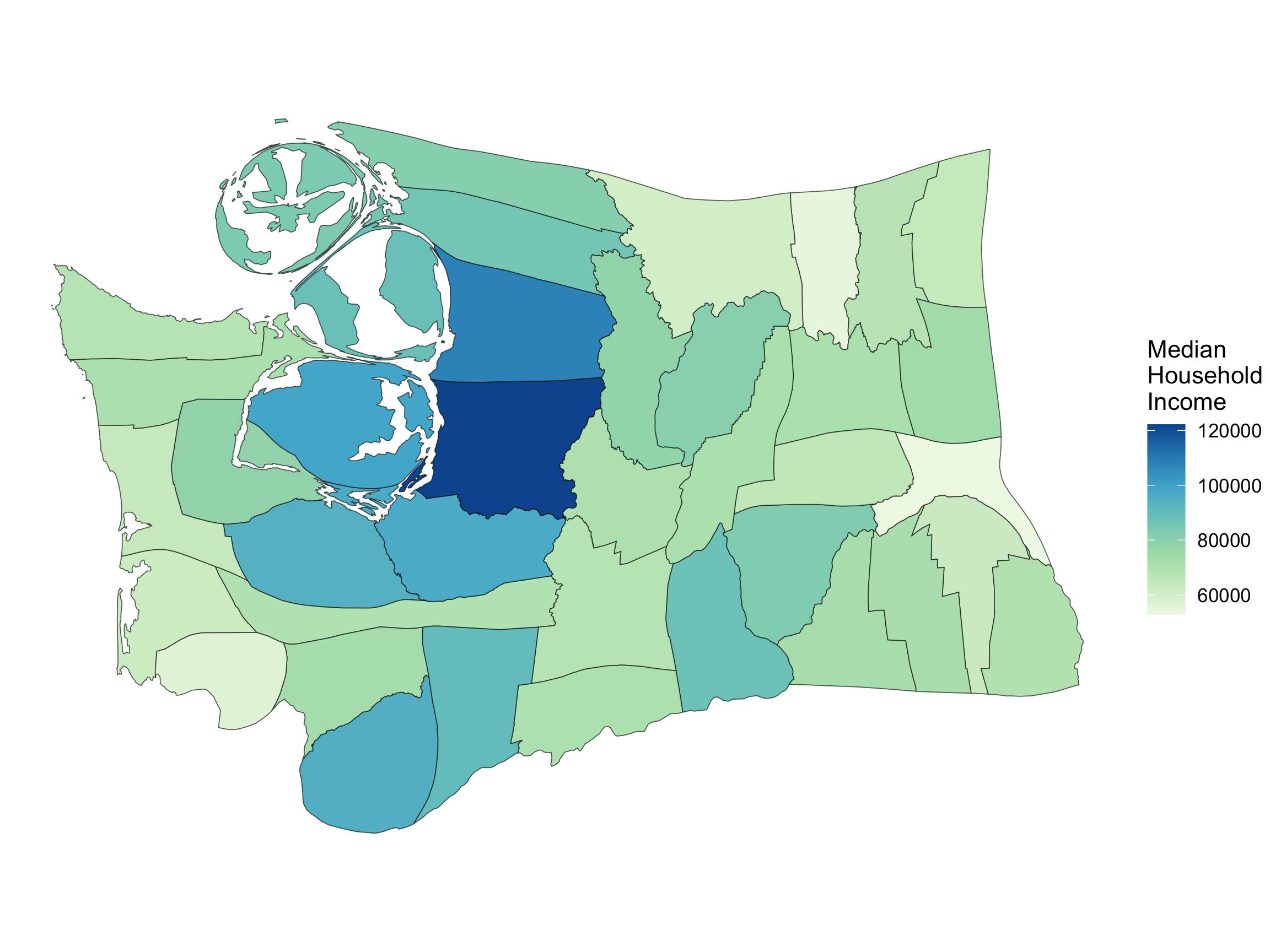
Different CRS -> Different Looking Map

Cartograms
Scale polygons by a variable.
Cartograms
Often scaled by a population size type variable.
wa_transf_pop <- wa_transf_pop %>%
  rename(population_size = value,
         median_income = estimate)

wa_transf_pop <- cartogram_cont(
  wa_transf_pop,
  weight = "population_size"
  )

ggplot() +
  geom_sf(data = wa_transf_pop,
          mapping =
            aes(geometry = geometry,
                fill = median_income)) +
  coord_sf() +
  scale_fill_distiller(
   name = "Median \nHousehold \nIncome",
   direction = 1, type = "seq", palette = 4) +
  theme_void()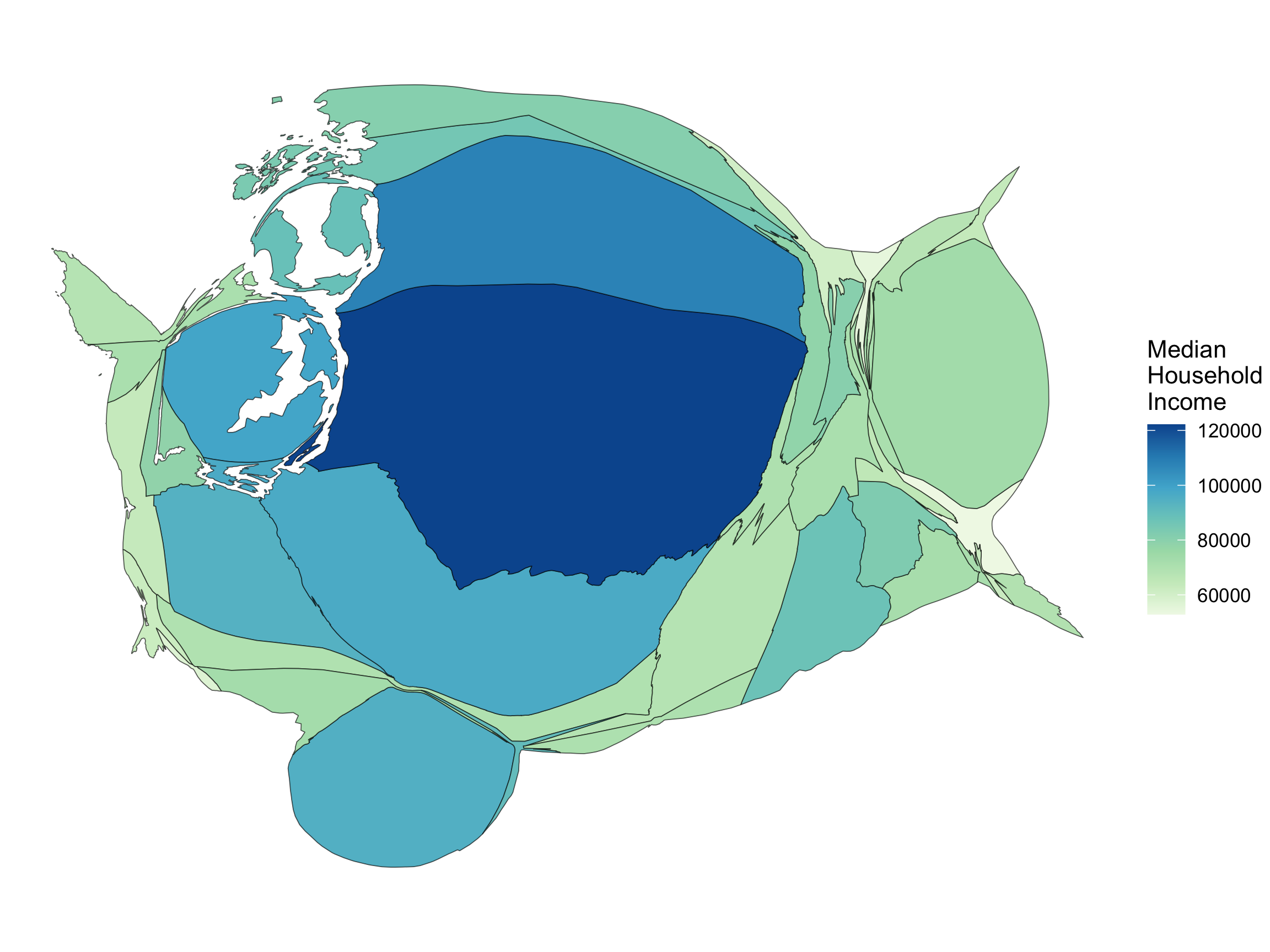
Hexbin Maps
Static Maps
- What if we want to zoom in?
Alluetian Islands
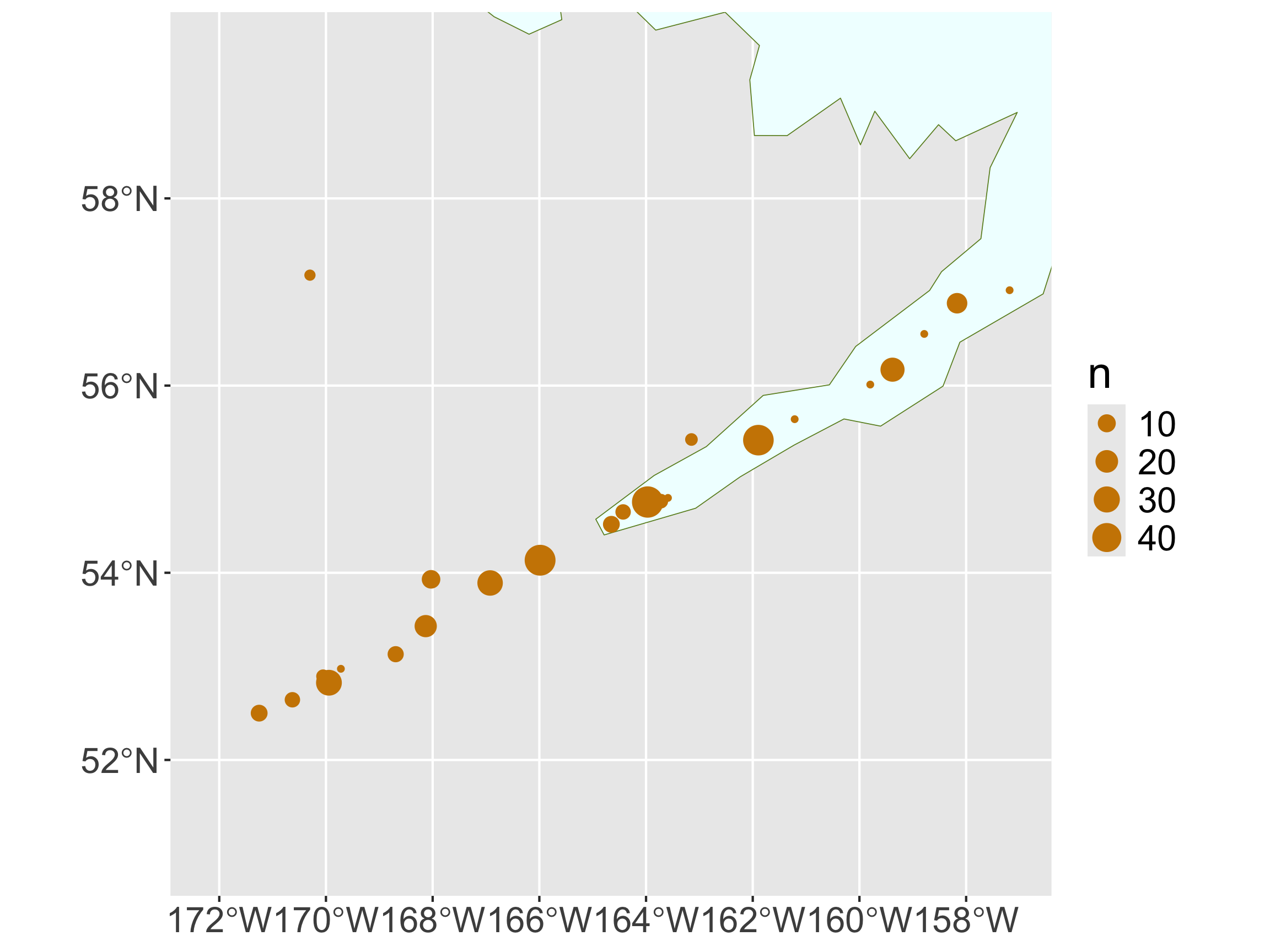
- Not a great base layer…
- What about dynamic zooming and clickable labels?