

Different Classes in R
Grayson White
Math 241
Week 7 | Spring 2026
Why do we need to talk about dates and times?
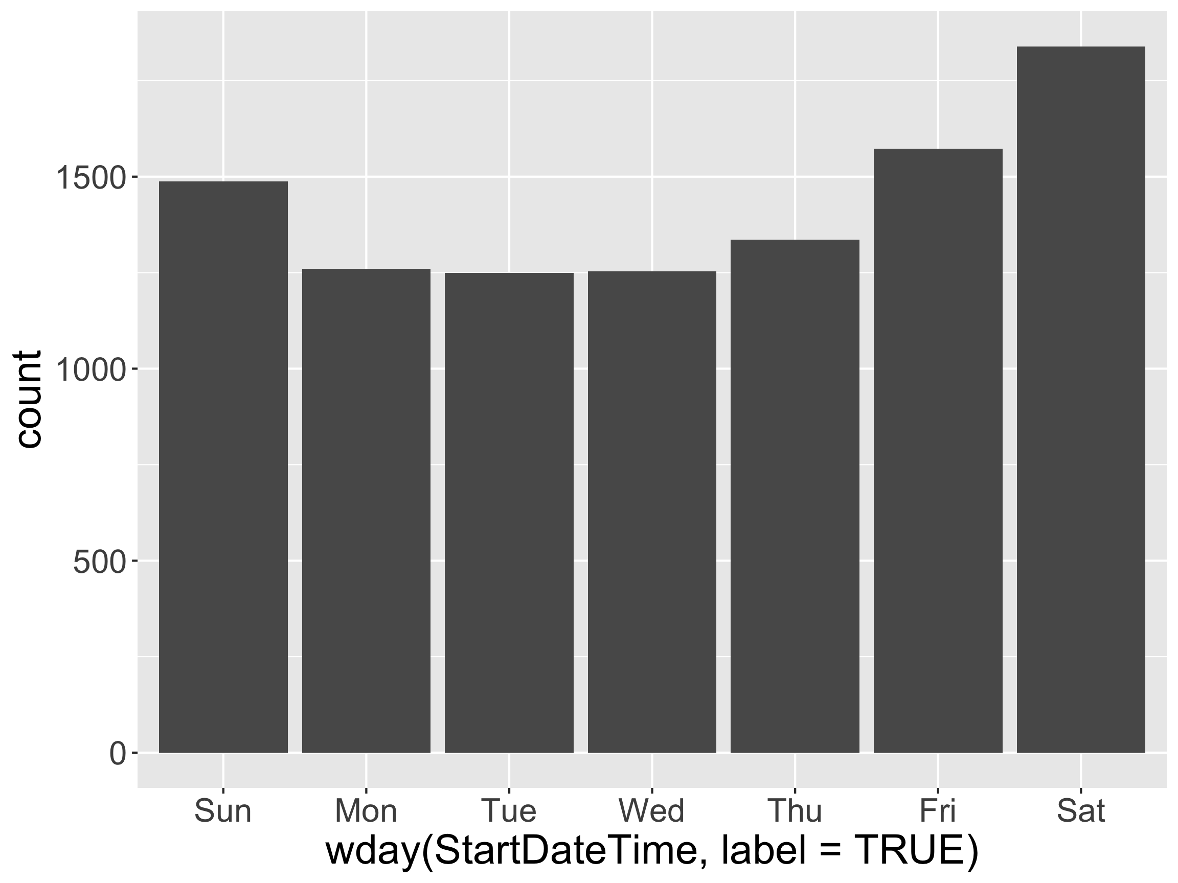
Question: When did the crashes happen?
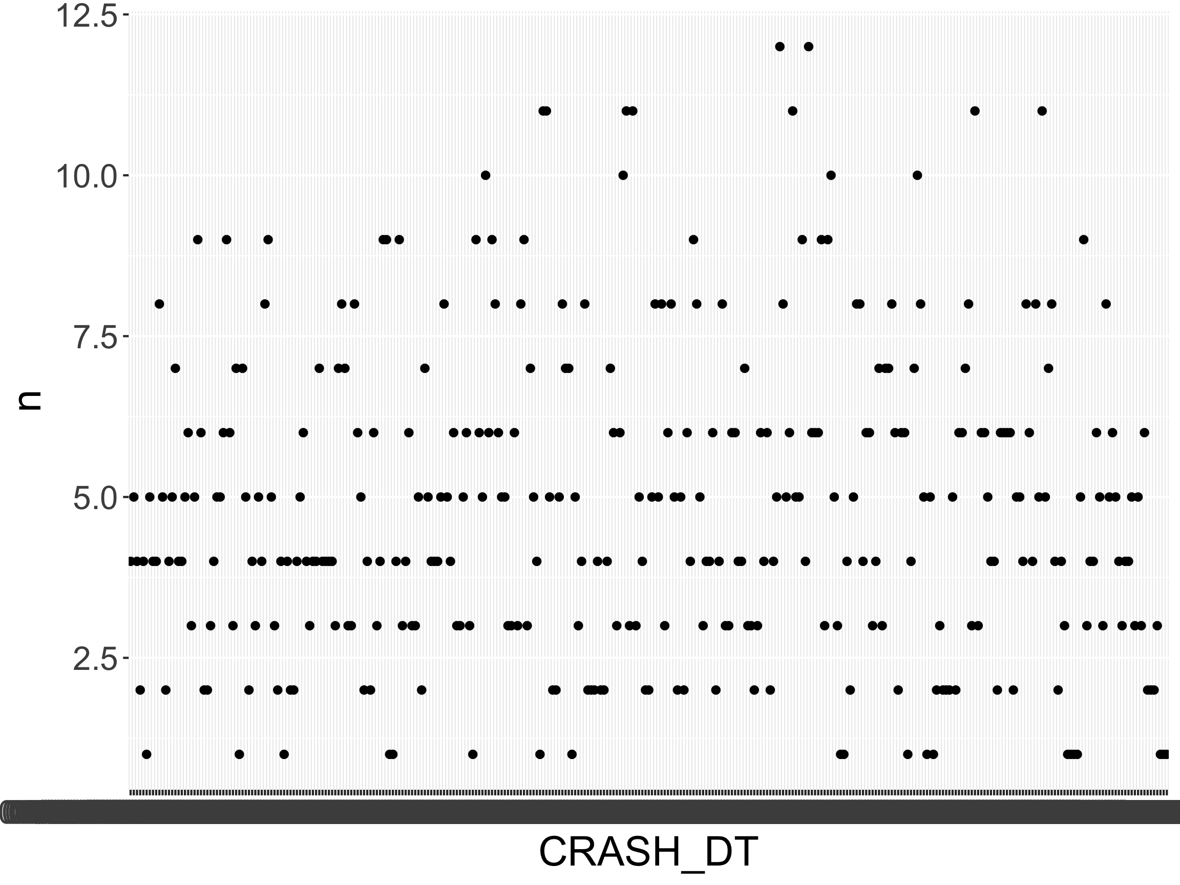
Why do we need to talk about dates and times?
Question: When did the crashes happen?
- Hard to see daily patterns. Switch time interval?
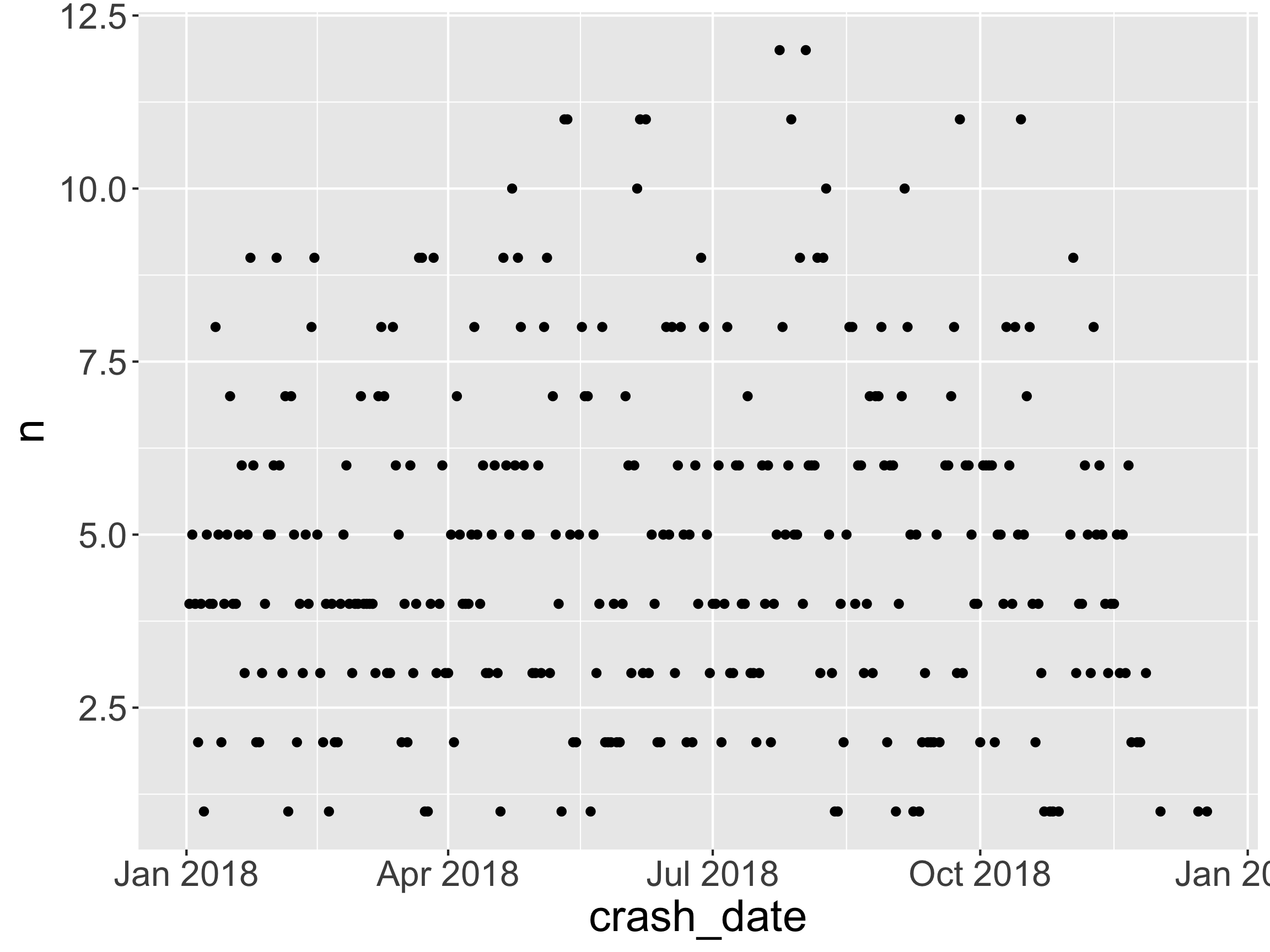
Why do we need to talk about dates and times?
Question: When did the crashes happen?
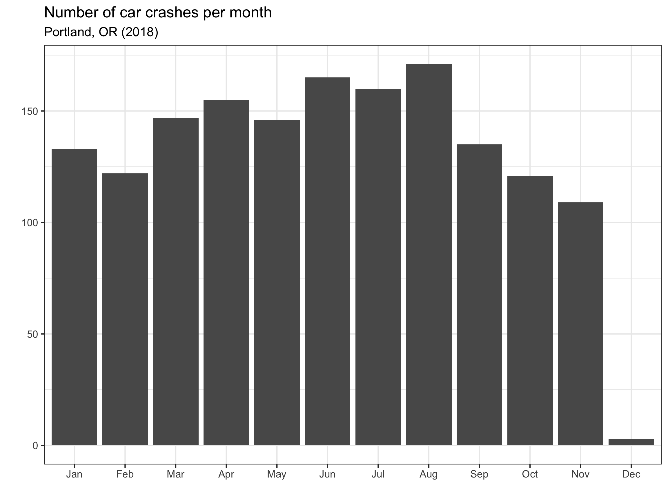
- Better! Chart junk?
Grabbing Components
Grabbing Components
Factors with forcats

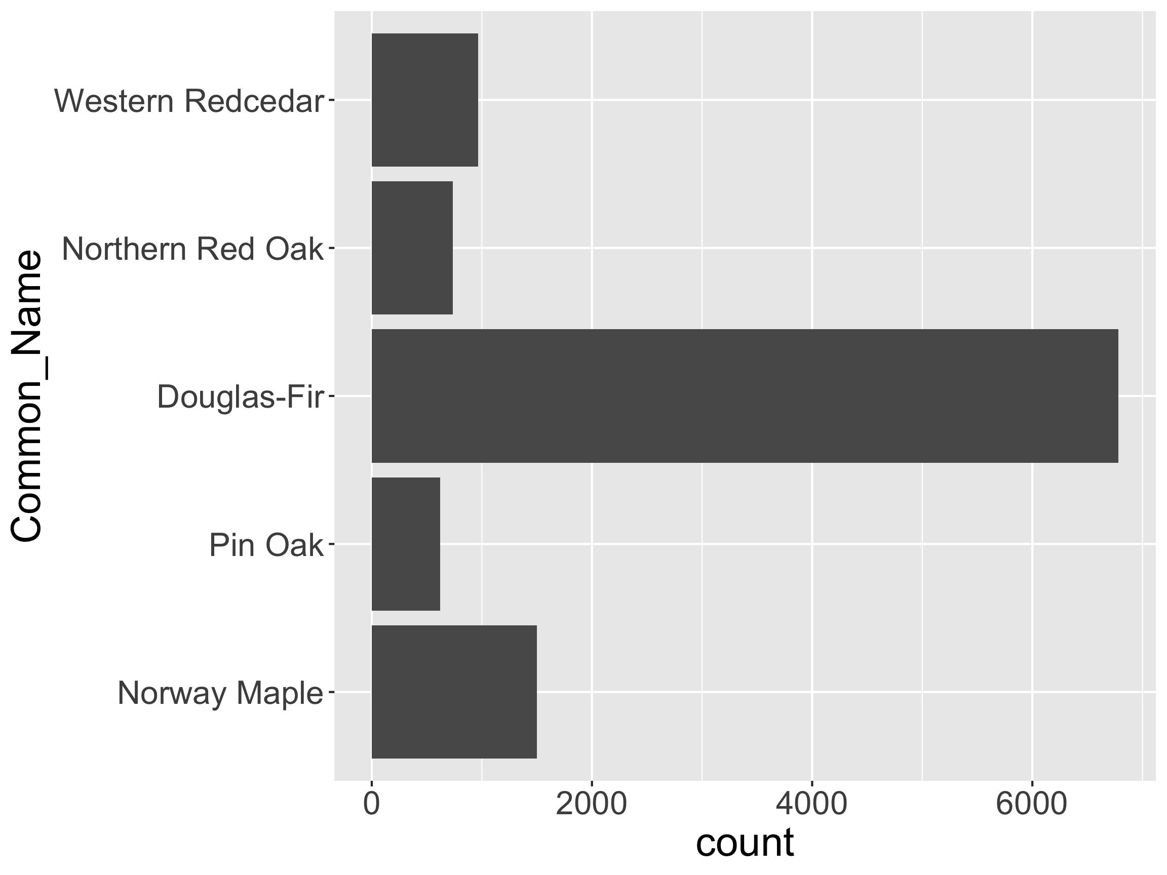
Motivation: Imposing Structure on Categorical Variables
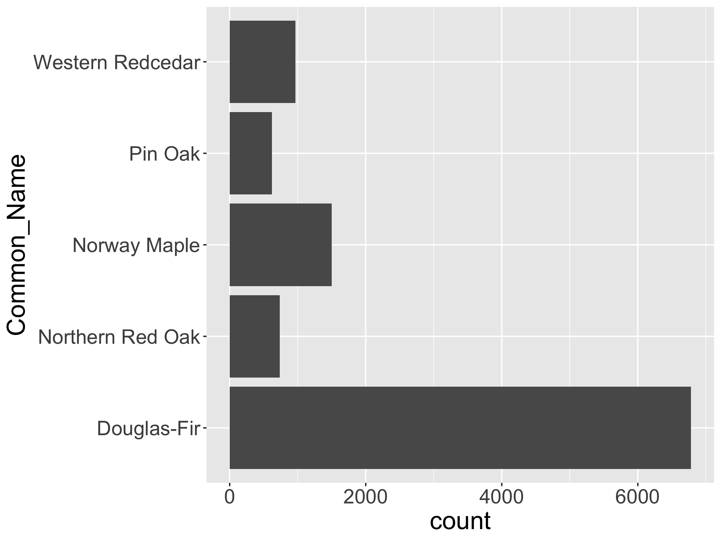
How might we want to restructure this graph?
Reorder the Levels
Note: This code didn’t permanently change the order in
pdxCommon. Why?How might we want to restructure this graph?
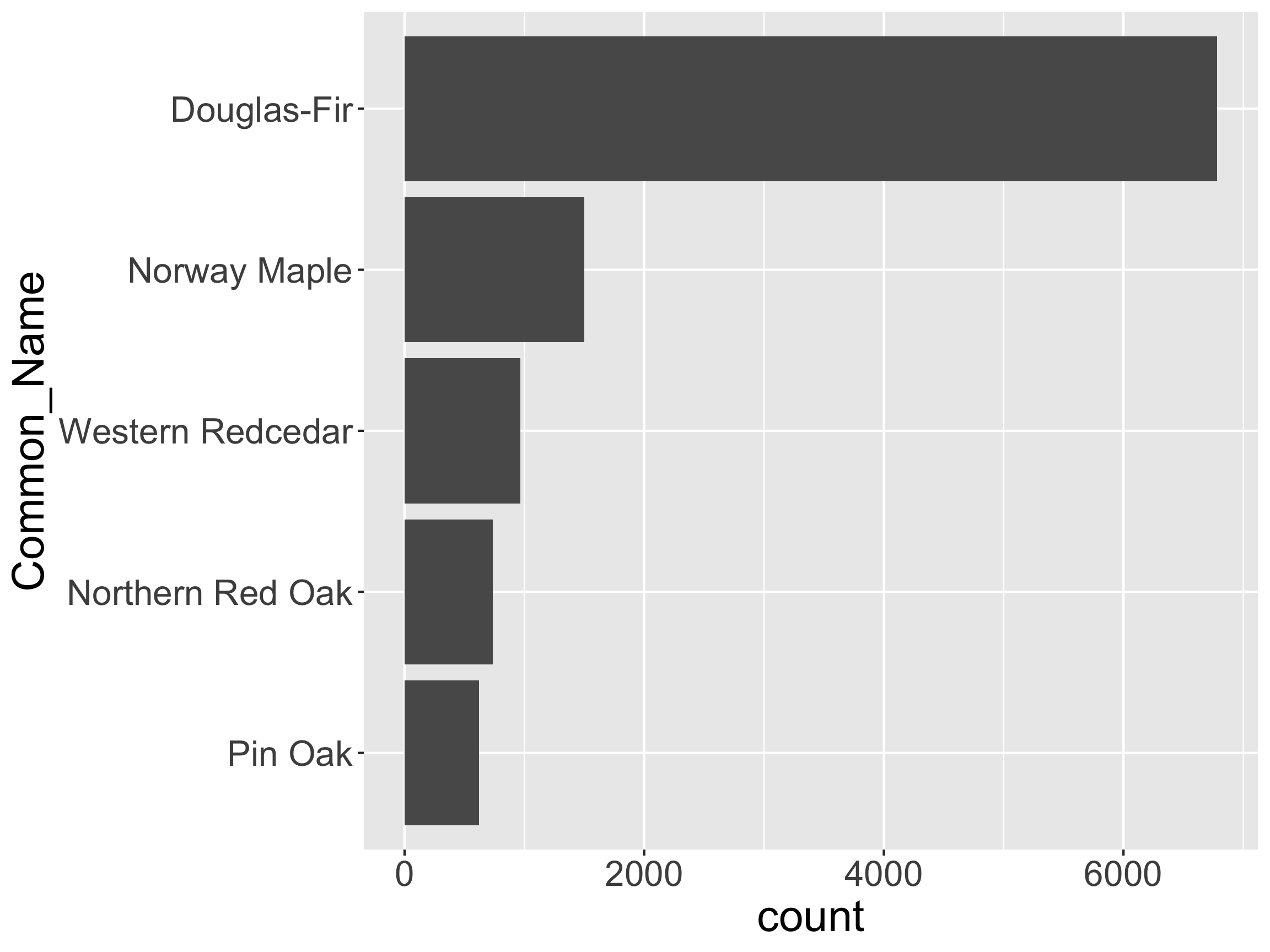
reverse the Levels

Or, If You Love the Pipe…
Reorder the Levels

- Can also relevel manually
Reorder the Levels
- Or maybe I just want to bring one or two category to the front
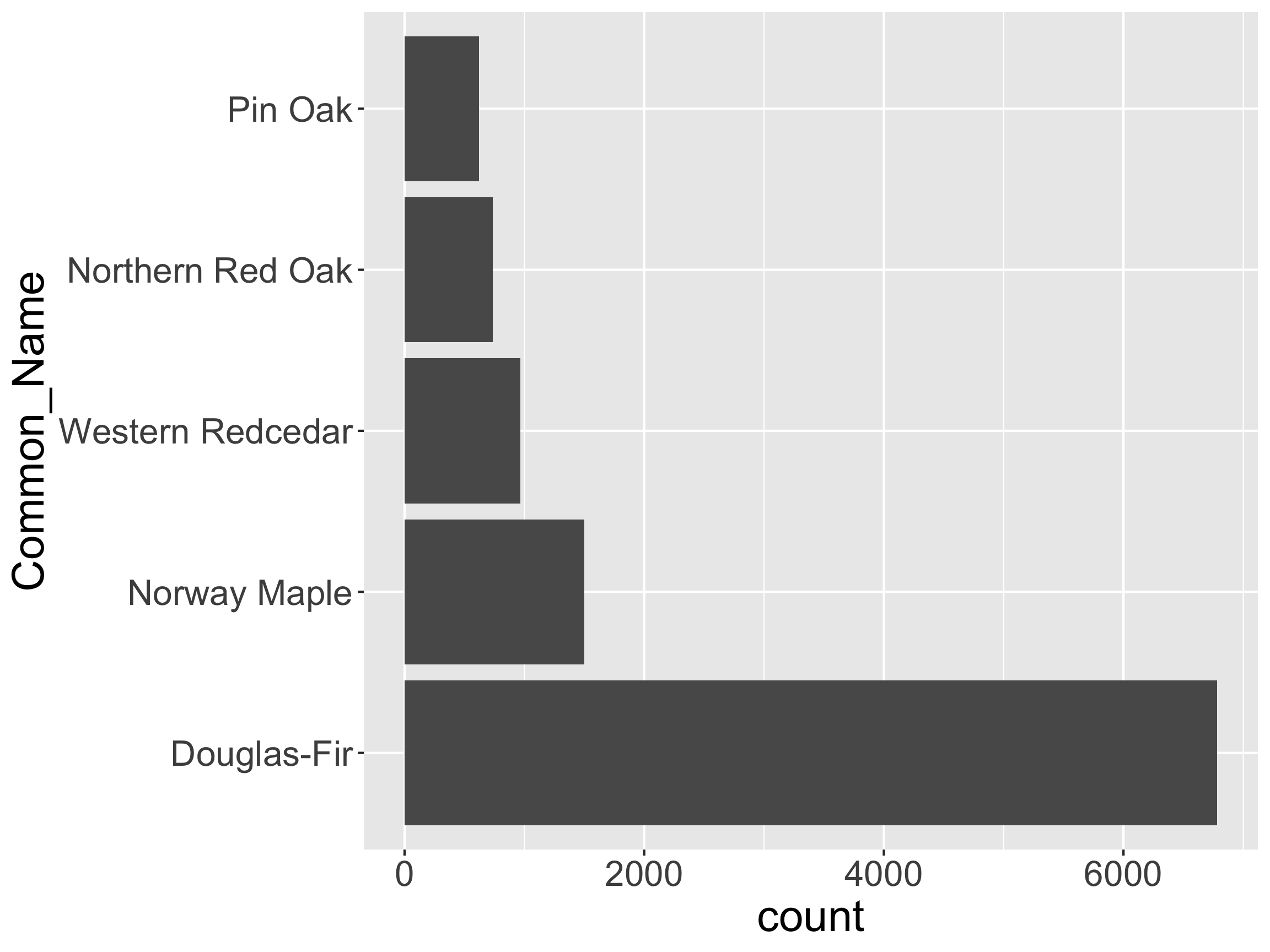
Reordering by Another Variable
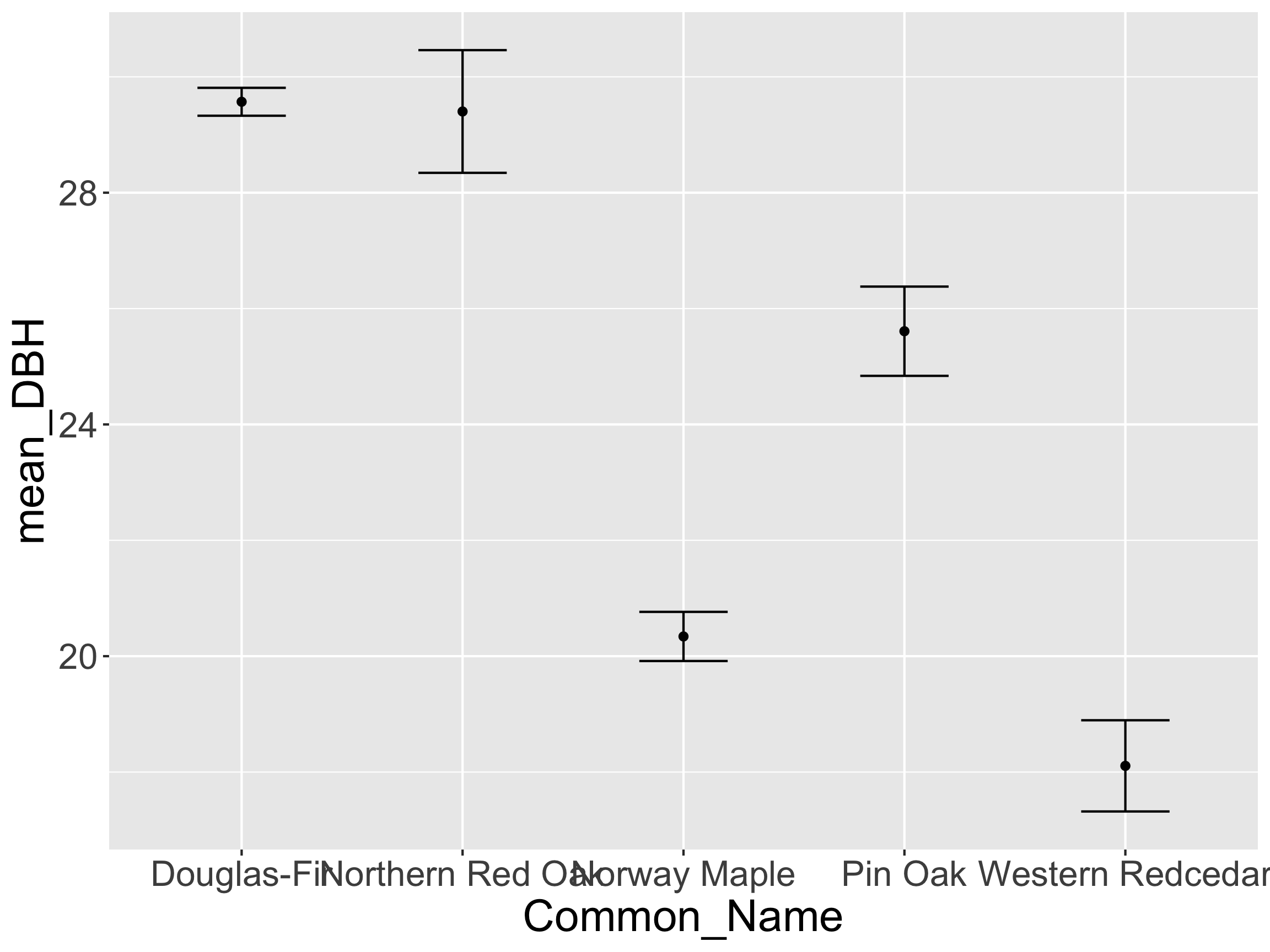
- How might we want to reorder
Common_Name?
Reordering by Another Variable
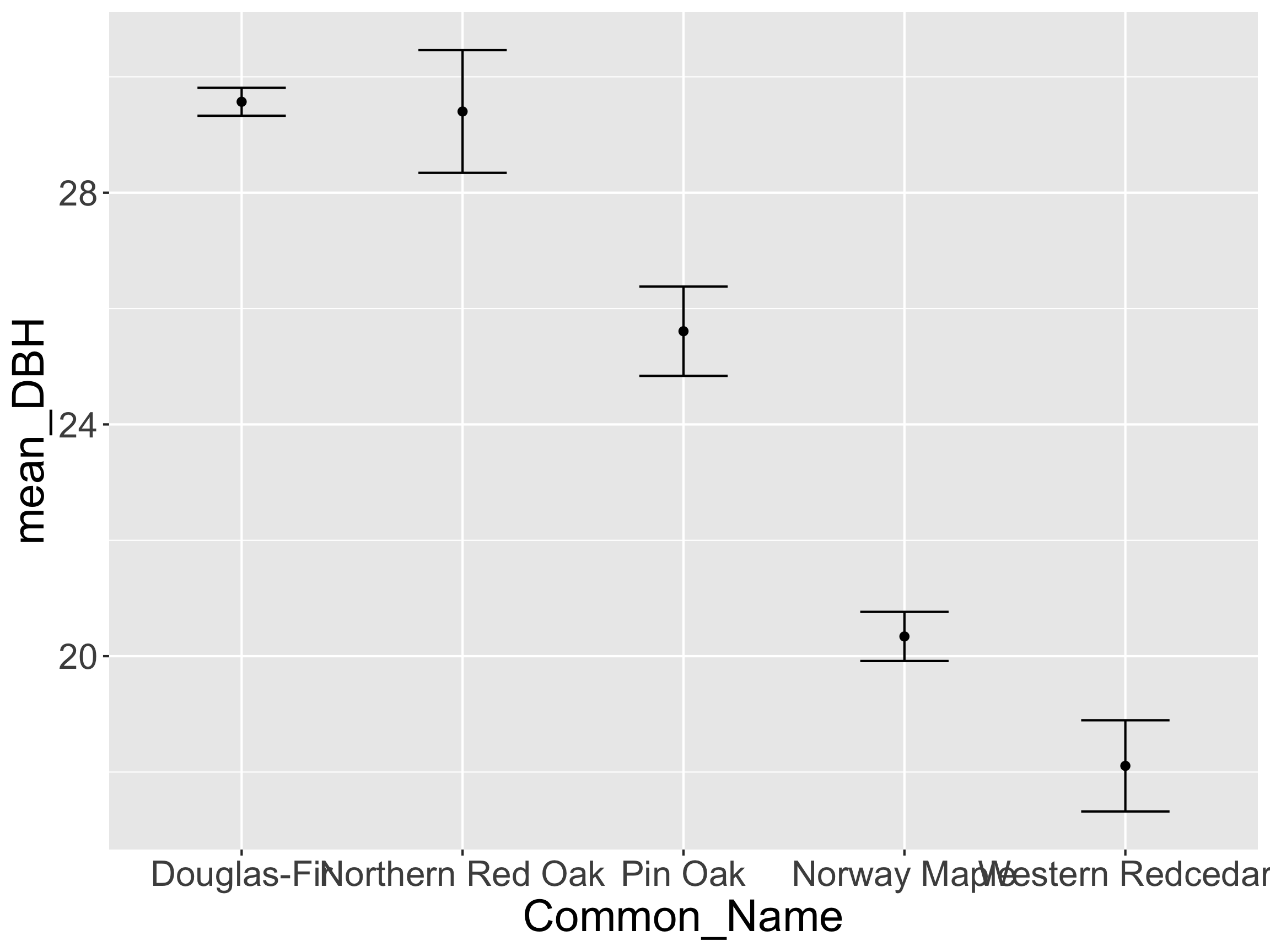
Reordering by Other Variables
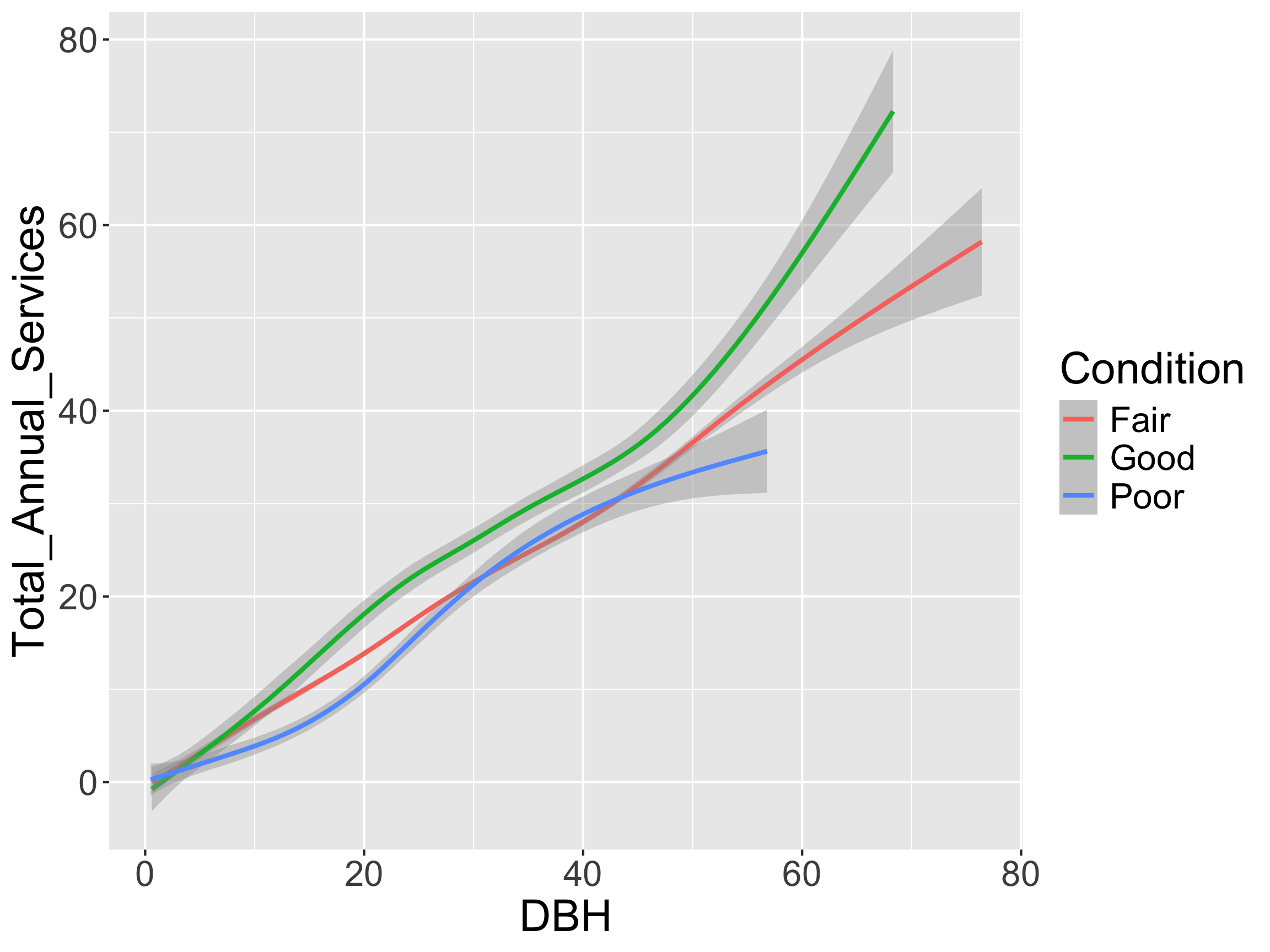
- How might we want to reorder
Condition?
Strings with stringr!
Our Toy Lyric
[1] "But I would walk 500 miles,"
[2] "And I would walk 500 more,"
[3] "Just to be the man who walks a 1000 miles,"
[4] "To fall down at your door" - Song?
- Artist?